
Evaluating AI-based Molecular Modelling with Physical Simulation
Published:
Introduction
In my last blog post, I explored Boltz-2 co-folding model applied to novel chemical modalities, including covalent macrocyclic molecular glue Elironrasib and its induced protein complexes. While the post received positive feedback, a detailed investigation was not performed. As both a computational chemist and a growing expert in cheminformatics, I believe it is crucial to analyse current AI models through a physics-based lens, leveraging corresponding data to inspire practical applications within the drug discovery industry.
This new article will serve as a supplement, specifically designed to address two key questions:
1. Which are those 'good' AI models that most closely approach physics as the ground truth, while also maintaining low computational cost?
2. Could physics effectively guide the identification, refinement, or even rescue of 'imperfect' AI models so far for molecular modelling?
Key Conclusions at the Beginning
A. Machine Learning Force Fields vs. Traditional Methods
The latest Machine Learning Force Fields (MLFFs), often based on Atomic Neural Network Potentials (NNPs), have achieved Quantum Mechanics (QM) level accuracy for small organic molecules. These models can serve as Density Functional Theory (DFT) surrogates effectively for rapid energy calculations. However, the speed of NNPs for molecular simulation remains significantly inferior to traditional force fields utilising classic parameters. Furthermore, the inherent architecture of NNPs may pose restrictions on their integration with advanced techniques for enhanced sampling, such as Hamiltonian replica exchange Molecular Dynamics (MD) or Metadynamics depending on the collective variable (CV) in physical quantity.
B. The Challenges of Post-processing AI Prediction with Statistical Mechanics
While traditional statistical mechanics methods are robust approximations of QM macroscopically and are capable of handling most challenging chemical systems, certain tricky cases (e.g., atropisomerism) need extreme caution. If an incorrect stereochemical scenario is generated by an AI model, the subsequent physical modelling and refinement process can become substantially more difficult to rectify.
C. Practical Impact of Machine Learning Models from Cheminformatics to Molecular Modelling
We observe mature machine learning models within cheminformatics dedicated to predicting atomic properties, offering significant, though often understated, benefits to computational chemistry workflows. There are some notable examples including graph-based pKa and charge models, which facilitate force-field parameterisation tasks and accelerate simulation pipelines efficiently.
D. The Role of Co-Folding and Physical Evaluation
While co-folding models can generate structural hypothesis rapidly (provided that the associated data and training overhead are disregarded), more expensive physical approaches are optimally suited for subsequent evaluation and identification of false positives, providing necessary inspection, refinement and understand that more closely serve Structure-Based Drug Design (SBDD).
Ligand Conformational Analysis in Solution
For small organic molecule drugs, solution-state conformations are critical, influencing both receptor binding events and pharmacokinetics (PK) properties. Computational and medicinal chemists frequently employ conformational control strategies to restrict or "lock" the bioactive state in solution. This approach is essential for reducing the entropic penalty and enhancing binding affinity for a specific target. For modalities that extend beyond the Rule of Five (bRo5), their folding behavior (often termed 'Chameleonicity') is equally crucial for achieving desired permeability and solubility.
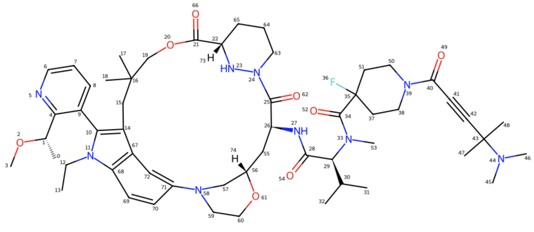
Following the work introduced in my previous article, I selected the macrocyclic molecular glue Elironrasib (Figure 1) again for a detailed solution-state conformational analysis. Herein, I assess the performance of several force fields, including popular atomic NNPs. The evaluation focuses on two key metrics: their simulation speed for conformational sampling and their energy accuracy relative to the established QM/DFT standard reference.
Choice of Sampling Approach
In molecular modelling, both the Monte Carlo (MC) and Molecular Dynamics (MD) algorithms are routinely employed for simulation studies. During my PhD few years ago, I frequently relied on MacroModel, a software based on the Metropolis MC algorithm (developed by the Still group and later acquired by Schrödinger), for sampling multiple conformational minima of small-molecule used in NMR structure elucidation. Coupled with the proprietary OPLSx force-field (which is originally built from the Jorgensen group), this method is highly effective for searching low-energy conformers in an implicit solution environment. Similarly for the protein modelling, there are MC-based softwares such as Rosetta which I often use to handle receptor structures when needed.
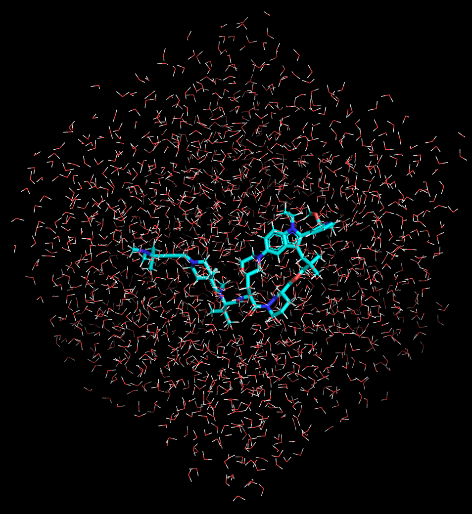
However, pure MC algorithms are primarily suitable for equilibrating and converging systems with limited degrees of freedom (e.g., rotamers) within the NVT ensemble, and they inherently struggle to reveal detailed kinetic information. Consequently, MC is typically applied to predict thermodynamic properties of the solute with an implicit solvation model. Over the years in industry, I have come to appreciate the critical importance of explicit water models for accurate Computer-Aided Drug Design (CADD) research. Therefore, the MD integrated with explicit solvation is preferentially chosen for conformational sampling in this study (Figure 2).
The comparison will focus on four representative force fields, encompassing both conventional and advanced ML approaches:
- General AMBER Force Field (GAFF) - A conventional, parameterised small-molecule force field, highly compatible with the widely used AMBER family of biopolymer force fields. This represents a traditional, established methodology and was used in my PhD work.
- SAGE (OpenFF-2.2.1) - The latest generation small-molecule force field released by the Open Force Field Initiative. SAGE employs the innovative SMIRNOFF framework for transferable parameterisation and is often benchmarked as outperforming GAFF.
- ANI2x - The pioneer Atomic Neural Network Potential (NNP) from the ANI family, developed by the Roitberg group. It supports the most common elements found in uncharged organic molecules.
- MACE - A modern class of NNPs that utilise advanced graph architecture to enhance both accuracy and computational efficiency. Its distilled small model has been selected for my simulation to maximise performance.
The greatest challenge in MD simulations is achieving ergodicity under the constraints of Newton's laws and the Langevin equation. To prevent the system from becoming trapped in local minima and to enhance conformational sampling significantly, I incorporated the Replica Exchange (REMD) algorithm, operating across temperatures exceeding 300 K, as well as the Solute Tempering (REST) technique through Hamiltonian modification.
However, these established enhanced sampling methods can only be applied to classic force fields that possess explicit, analytically defined terms for bonding and non-bonding interactions. In NNPs, the energy and gradient forces are calculated through a complex forward pass of the atomic position features within the neural network's 'black box' (Text 3). This process, analogous to methods like ETKDG conformer generation that is biased by 'distance constraints' matrices derived from crystallography, lacks an easily modulated analytic Hamiltonian function. Consequently, it is difficult to modify the system Hamiltonian directly in theory as required in REST technique. Furthermore, subjecting the system to high temperatures poses a significant risk of thermal instability under NNPs, as the majority of their training data consists of QM/DFT geometries minimised typically at 0 K and/or in vacuum for the zero-point energy, lacking explicit thermal and/or environmental correction.
class HybridNNP(torch.nn.Module):
    def __init__(self, atomic_numbers, ml_atoms):
        super().__init__()
        self.indices = torch.tensor(ml_atoms, dtype=torch.long, device=device)
        self.atomic_numbers = torch.tensor(atomic_numbers, device=device).unsqueeze(0)
        self.model = ANI2x(periodic_table_index=True)
        self.model.to(self.atomic_numbers.device)
    def forward(self, positions):
        positions = positions.to(self.atomic_numbers.device)
        positions = positions[self.indices]
        positions = positions.unsqueeze(0).float() * 10 # nm -> Å
        result = self.model((self.atomic_numbers, positions))
        energy = result.energies[0] * 2625.5 # Hartree -> kJ/mol
        return energy
A further significant challenge arises from the charged state of organic small molecules in solution. Elironrasib contains a tertiary amine located near its covalent warhead. Based on the pKa prediction from pkasolver model (Figure 4), this nitrogen atom should be preferentially protonated in water at physiological pH around 7.4. However, most current atomic NNPs, including the ANI2x and MACE models tested in this study, are restricted to neutral molecules. To maintain a feasible and direct comparison across all methods, I had to exclude such more biologically relevant protonation/charge from the simulation. Although this might introduce certain limitation to the accuracy, corresponding parameterisation become easier for classical force fields in this case.

Due to the lack of PLUMED plugin compilation with GROMACS installed in my local machine (a PC with 16 CPU cores, 16 GB RAM, and an RTX5070 GPU), the REST simulation and metadynamics mentioned later were performed using OpenMM and its extension tools. In practice, there was no significant difference in simulation speed between these two open platforms, though I noted they feel slightly slower than commercial software like Desmond which is developed by D. E. Shaw and optimised by Schrödinger for industrial use. Anyway we have modules like ParmEd and OpenFF interchange to convert topology in different formats.
One challenge, however, lies in integrating explicit water models (TIP3P in this study) with the organic solute when using NNPs. Traditionally, accurate solvation modelling is achieved via the QM/MM approach with electronic embedding at the boundary (a principle emphasised by Adrian during my PhD in Bristol). Considering both the necessary computational speed and the NNPs characteristics, ML/MM with mechanical embedding was chosen as the alternative approach for this study as guided by a tutorial from OpenMM workshops. To construct this ML/MM system, most of the classical parameters governing the solute (i.e., bonds, angles, torsions, non-bonded terms) must be removed (Text 5) and entirely replaced by the atomic NNPs (Text 3).
def removeBonds(system, atoms, removeInSet=True, removeConstraints=True):

    atomSet = set(atoms)
    import xml.etree.ElementTree as ET
    xml = mm.XmlSerializer.serialize(system)
    root = ET.fromstring(xml)

    def shouldRemove(termAtoms):
        return all(a in atomSet for a in termAtoms) == removeInSet

    for bonds in root.findall("./Forces/Force/Bonds"):
        for bond in bonds.findall("Bond"):
            bondAtoms = [int(bond.attrib[p]) for p in ("p1", "p2")]
            if shouldRemove(bondAtoms):
                bonds.remove(bond)
    for angles in root.findall("./Forces/Force/Angles"):
        for angle in angles.findall("Angle"):
            angleAtoms = [int(angle.attrib[p]) for p in ("p1", "p2", "p3")]
            if shouldRemove(angleAtoms):
                angles.remove(angle)
    for torsions in root.findall("./Forces/Force/Torsions"):
        for torsion in torsions.findall("Torsion"):
            torsionAtoms = [int(torsion.attrib[p]) for p in ("p1", "p2", "p3", "p4")]
            if shouldRemove(torsionAtoms):
                torsions.remove(torsion)

    if removeConstraints:
        for constraints in root.findall("./Constraints"):
            for constraint in constraints.findall("Constraint"):
                constraintAtoms = [int(constraint.attrib[p]) for p in ("p1", "p2")]
                if shouldRemove(constraintAtoms):
                    constraints.remove(constraint)

    return mm.XmlSerializer.deserialize(ET.tostring(root, encoding="unicode"))


def removeMMInteraction(system, ml_atoms):
    newSystem = removeBonds(system, ml_atoms)
    for force in newSystem.getForces():
        if isinstance(force, mm.NonbondedForce):
            for i in range(len(ml_atoms)):
                for j in range(i):
                    force.addException(ml_atoms[i], ml_atoms[j], 0, 1, 0, True)
        elif isinstance(force, mm.CustomNonbondedForce):
            existing = set(tuple(force.getExclusionParticles(i)) for i in range(force.getNumExclusions()))
            for i in range(len(ml_atoms)):
                a1 = ml_atoms[i]
                for j in range(i):
                    a2 = ml_atoms[j]
                    if (a1, a2) not in existing and (a2, a1) not in existing:
                        force.addExclusion(a1, a2, True)
    return newSystem
Following extensive trials in parameterisation and testing, the performance of the diverse simulations conducted on Elironrasib is summarised below:
| Methods | Ensembles | Timescale | Stepsize | Constraints | Enhancement | Platform | Speed |
|---|---|---|---|---|---|---|---|
| GAFF | NPT 300 K | 10 ns | 2.0 fs/step | H-bond | None | OpenMM | 465 ns/day |
| SAGE | NPT 300 K | 10 ns | 2.0 fs/step | H-bond | None | OpenMM | 460 ns/day |
| ANI2x | NPT 300 K | 200 ps | 0.5 fs/step | None | None | OpenMM | 1.3 ns/day |
| MACE_small | NPT 300 K | 100 ps | 0.5 fs/step | None | None | OpenMM | 0.72 ns/day |
| SAGE (REMD) | NPT with 16 replica 300-475 K | 10 ns | 2.0 fs/step | H-bond | 10000 MC exchange attempts | GROMACS | 35 ns/day/rep |
| SAGE (REST) | NPT with 16 replica 300-600 K | 10 ns | 2.0 fs/step | H-bond | 10000 MC exchange attempts | OpenMM | 21 ns/day/rep |
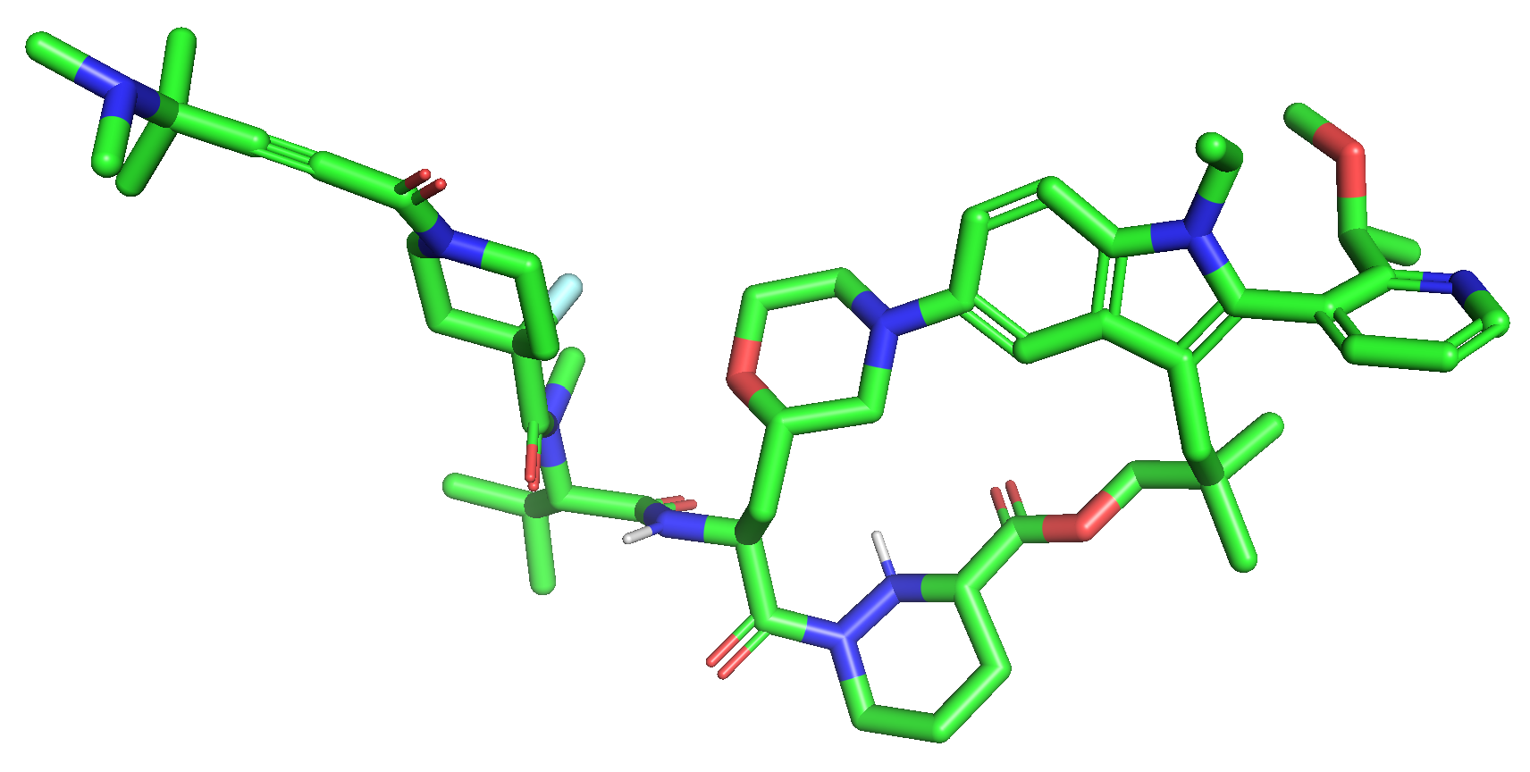
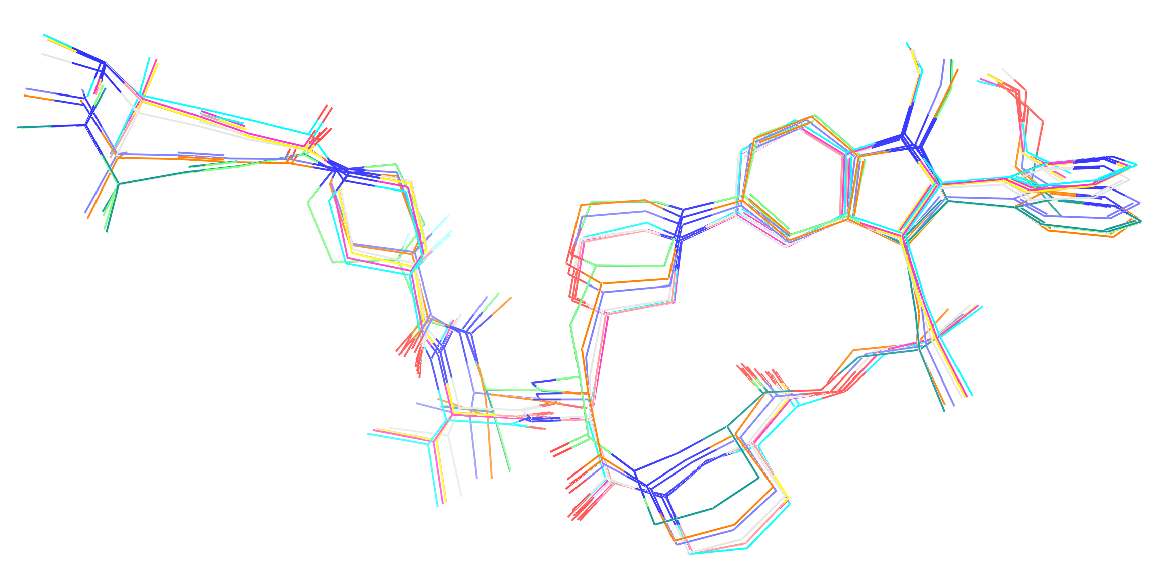
The performance data in table 6 clearly demonstrates that the operational simulation speed of the two NNPs is orders of magnitude slower than that of the classical force fields. This gap is notable, even when considering that the classical methods required additional time for BCC atomic charge parameterisation (using the semi-empirical AM1 protocol) on Elironrasib's 150+ atoms at the beginning. Given the limited timescales, particularly for the NNPs, these models are expected to sample only a narrow set of geometries distinct from the initial bioactive state (Figure 1).
However, two core questions remain in my mind:
Which of these simulations is most efficient at sampling low-energy conformers?
Was any significant conformational change observed during the landscape exploration?
Evaluation with Quantum Mechanics Calculations
To address the first core question - the relative quality of the simulation methods, it is essential to benchmark the sampled geometries against a high-level quantum mechanical standard (Figure 7). This required significant post-processing efforts: Up to 1000 snapshots were extracted from each simulation, and the Elironrasib solute geometry from each was minimised using the semi-empirical XTB method under the implicit ALPB solvation model.
Based on my experience in QM calculations, this level of initial optimisation is sufficient before proceeding to single-point energy (SPE) calculation at the higher Density Functional Theory (DFT) level. This is because geometry is generally less sensitive to basis set than energy is, and semi-empirical methods are often adequate for preliminary optimisation tasks.
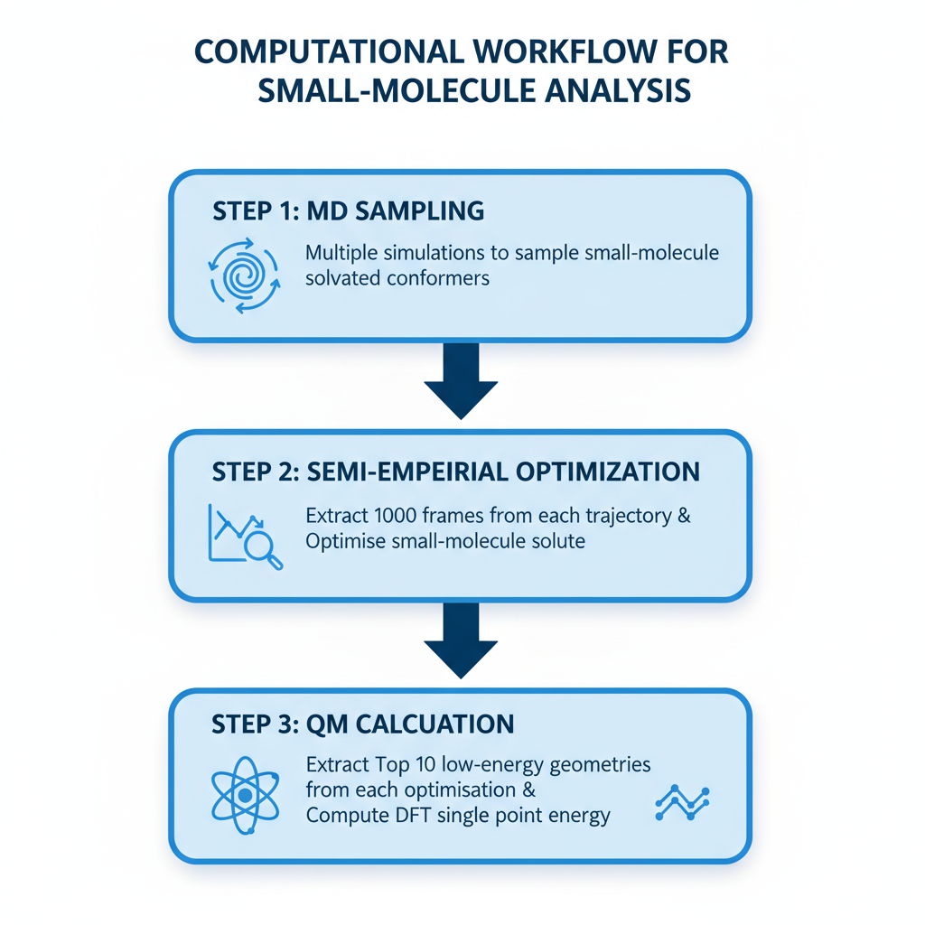
Despite XTB being significantly faster than full DFT for the initial guess and Self-Consistent Field (SCF) calculation iterations, completing thousands of ensemble optimisations feasibily in a day on PC still need me to loosen the convergence criteria. As demonstrated by the test on the Elironrasib bioactive conformation (Figure 8), the error introduced by such quick minimisation is acceptable. This reflects a crucial lesson for me learnt in the biotech industry so far: It is often necessary and reasonable to sacrifice a small degree of accuracy for overwhelming gains in efficiency.
| XTB opt. convergence criteria | aligned best rms | relative XTB opt. energy (+ ALPB) | relative DFT SPE by looseSCF (+ CPCM) | relative DFT SPE by NormSCF (+ CPCM) |
|---|---|---|---|---|
| extreme | 0.000 Å | 0.000 kcal/mol | 0.087 kcal/mol | 0.000 kcal/mol |
| vtight | 0.042 Å | 0.003 kcal/mol | 0.124 kcal/mol | 0.038 kcal/mol |
| tight | 0.791 Å | 0.471 kcal/mol | 1.647 kcal/mol | 1.561 kcal/mol |
| normal | 0.777 Å | 0.872 kcal/mol | 1.350 kcal/mol | 1.261 kcal/mol |
| lax | 1.077 Å | 2.039 kcal/mol | 2.123 kcal/mol | 2.036 kcal/mol |
| loose | 1.230 Å | 2.673 kcal/mol | 1.818 kcal/mol | 1.734 kcal/mol |
| sloppy | 1.235 Å | 2.748 kcal/mol | 1.960 kcal/mol | 1.876 kcal/mol |
| crude | 1.264 Å | 3.471 kcal/mol | 2.321 kcal/mol | 2.238 kcal/mol |
| ff_original | 1.310 Å | 35.625 kcal/mol | 20.528 kcal/mol | 20.456 kcal/mol |
For DFT SPE calculation on the minimised conformers, my preferred methodology is wB97X(D3bj)/def2-TZVP - a range-separated hybrid functional with dispersion correction under a triple-zeta basis set. I remember this was recommended by the Grimme group for calculating mid-sized systems (> 100 atoms) with significant non-covalent interactions (addressing a common weakness of methods like B3LYP). Although no expensive diffusion function was added in the basis set, this method accurately reproduced solution-state NMR data for my PROTAC folding studies few years ago. Furthermore, I am encouraged to see similar DFT methods now being used by the MACE and Meta FAIR Chemistry teams to generate the OMol database for training their NNPs. Due to computational resource limitations, the SCF convergence criteria in ORCA was set to 'loose' (i.e., 10^-5 a.u. change in energy, and also RMS if an optimiser like DIIS is added) in order to quickly obtain each Elironrasib conformer’s SPE (approx. 20-30 minutes per conformer on my PC). While this is a low standard compared to Gaussian's typical 10^-7 a.u. default, such 'loose' criteria in ORCA is identical to the default quick setting in Jaguar and corresponding energy result closely approaches to the 'normal' mode (10^-6 a.u.) in this study (Figure 8).
Efficiency on Elironrasib Conformational Sampling and Energy Estimation
To address the efficiency of low-energy conformer generation, I first analysed the results using an Empirical Cumulative Distribution Function (ECDF) plot at XTB level (Figure 9 left). This plot clearly indicates that the majority of low-energy Elironrasib conformers were sampled from classical mechanics combined with enhanced simulation techniques. Specifically, the SAGE force field powered by REST proved most effective, yielding the most stable geometries identified by XTB minimisation.
To establish the QM standard feasibly, the 10 lowest energy XTB-optimised conformers from each simulation approach were subjected to DFT SPE calculation coupled with CPCM correction. A strong correlation was observed between the XTB semi-empirical energies and the final DFT energies under the implicit solvation model (Figure 9 right). Moreover, the majority of the lowest energy conformers, as ranked by DFT, were still sourced from the highly efficient REST sampling utilising the classic SAGE force field.

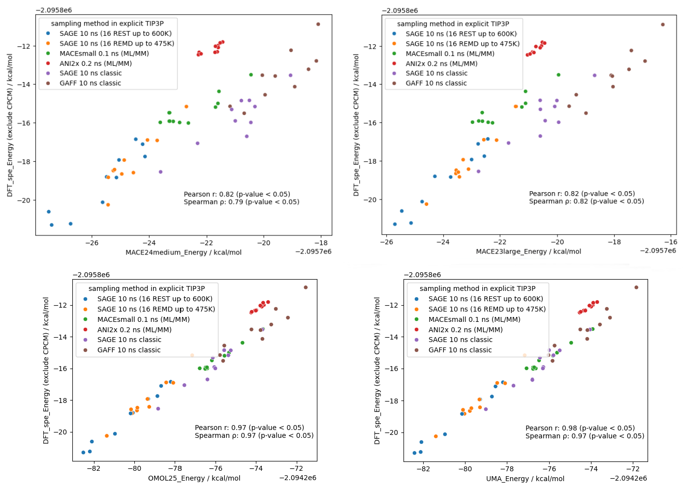
Benchmarking Larger NNP Models
Using these XTB-optimized geometries and DFT SPE, I then evaluated their energies against four larger NNP models (i.e., MACE and UMA trained on the OMol datasets released in recent years). Because most current NNP models do not yet support explicit solvent correction terms, the CPCM component was necessarily excluded from the DFT reference calculation to ensure a valid comparison.
The results are striking as shown in Figure 10 - these NNPs achieve incredible proximity to DFT accuracy, particularly the latest UMA/OMol25 models, meanwhile completing the SPE task in mere seconds.
This evidence strongly supports the announcement made by the Meta FAIR Chemistry team: Machine Learning Force Fields (MLFFs) are poised to become a true DFT surrogate for computational chemistry. Moving forward, I anticipate and look forward to the development of more AI models designed to accelerate continuum solvation calculations based on surface electrostatics and cavity, approaching PCM or COSMO accuracy.
Hydrophobic Collapse and Atropisomerism for Elironrasib
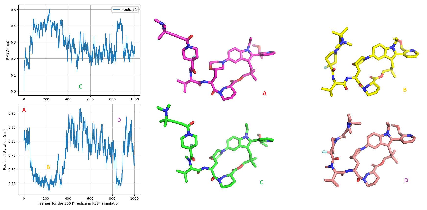
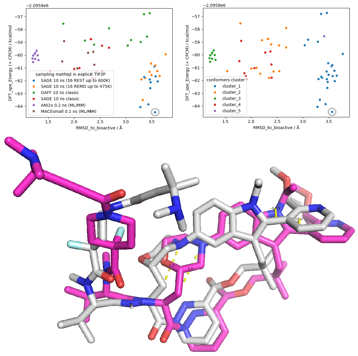
Double-checking the simulation trajectory with RMSD (Root Mean Square Deviation) and Radius of Gyration (Rg) plots (Figure 11 upper), I observe that the REST enhanced sampling effectively explored more compact geometries of Elironrasib compared to the initial bioactive state (magenta stick A). This collapse is a result of the linker branch (containing the covalent alkyne warhead for KRAS G12C) folding back and interacting with the macrocyclic core. This key folding state is also identified as the current global minimum among the conformational ensembles estimated by DFT calculated energy (grey stick, Figure 11 lower).
In addition to this collapse, a morpholine ring flip was also observed, shifting from an equatorial state (with a distance of 3.9 Å) to an axial state (with a distance of 3.0 Å), as indicated by the change in distance between the aniline tertiary-nitrogen and the substituted beta-carbon atoms. Nevertheless, the intramolecular hydrogen bond (IMHB) between the morpholine oxygen and the adjacent amide, as proposed in Revolution Medicines' publication, was hardly observed in the simulations performed here in water.
Notably, conformational exchange was never observed on the bi-aryl torsion — such motif was erroneously predicted by the co-folding model in my previous article. Given the significant steric bulk of the two aromatic rings, Elironrasib was suspected to possess atropisomerism (Figure 12). To investigate this, I re-ran the ligand REST simulation, starting from the 'other atropisomer' previously generated by Boltz-2, but again, no exchange across the torsional barrier occurred. This observation was ultimately confirmed by the literature: Elironrasib exists as a specific, stable atropisomer.
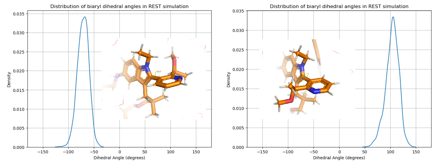
In classical MD at 300 K, typical kinetic barriers within 15 kJ/mol can often be overcome in timescales allowed. Enhanced sampling techniques like REST, when applied carefully, can boost this range up to approximately 15 kcal/mol. For example, this energy range might occasionally allow the observation of cis isomerisation from trans-amide, provided that the force field's torsional potential is not over-fitted harmonically. However, atropisomerism features energy barriers typically exceeding 25 kcal/mol (as reliably elucidated by NMR experiments or QM scans). Due to the extremely slow conversion rates governed by the Eyring equation, we chemists treat atropisomers as distinct, isolable compounds; Indeed, some KRAS Switch-II inhibitors currently in clinical trials are stable atropisomers with reported half-lives over decades.
This study provides me with a critical insight: There are fundamental mistakes made by current AI models that cannot be easily rescued or corrected by physical modelling. For advanced development, generative AI models must evolve to incorporate a deeper, more human-level understanding of science especially the awareness of stereochemistry over sequence for accurate structure prediction.
Highly Flexible Elironrasib Ligand Bound with CYPA
The Indication from Unbiased MD Analysis
Given the diverse set of conformations Elironrasib explores when free in solution, its CYPA-bound state became the next critical focus of this study. According to my previous blog, the Boltz-2 diffusion model generated a variety of co-folding hypothesis for the CYPA binary complex. Even though the stereochemistry and atropisomerism predictions were largely incorrect, the diffusion results suggested that both the KRAS binding motif and the G12C warhead branch of Elironrasib might retain significant flexibility when exposed to the solvent while bound to CYPA — a characteristic often seen in hetero-bifunctional molecules. I committed to validating such hypothesis using rigorous physics-based simulations in this follow-up post.
Starting from the ternary complex crystal structure (PDB: 9BFX), the KRAS G12C protein and its corresponding covalency were computationally removed to simulate the CYPA binary complex in solution. For comprehensive sampling, the system was replicated 20 times, each initiated with different velocities (10 replicas run with GROMACS and 10 others using OpenMM).
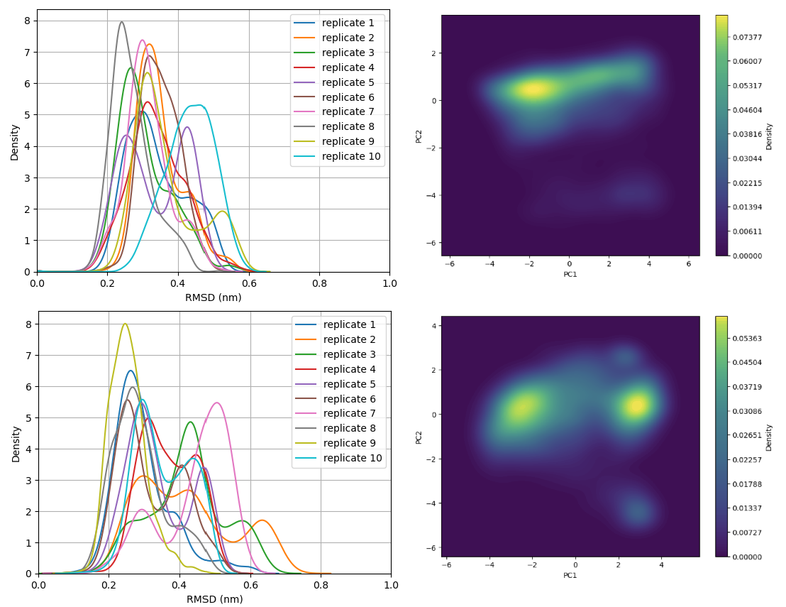
Analysis of both the RMSD distribution and the Principal Component (PCA) density revealed that no single conformational state converged or became significantly populated (Figure 13 upper). Each 10 ns pathway appears to visit a unique conformational space, clustering into three major ensembles (Figure 13 lower). The observation is clear - The Elironrasib linker warhead exhibits substantial dynamic motion in the absence of KRAS G12C. Furthermore, the exchange of atropisomer was, once again, not observed on Elironrasib even it was embraced within the CYPA binding pocket.
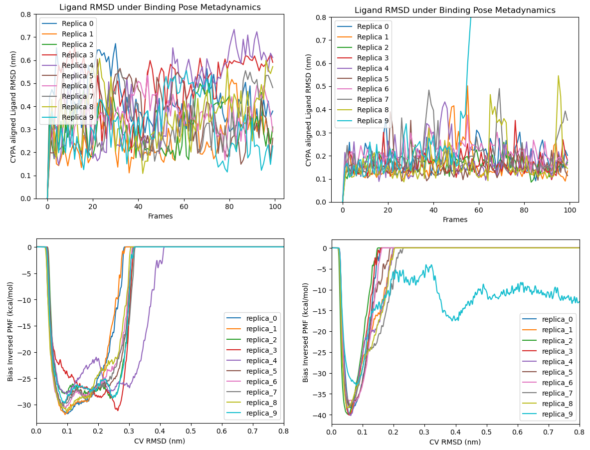
Further Confirmation through Binding Pose Metadynamics (BPMD)
To overcome the inherent sampling limitations of conventional MD, the Binding Pose Metadynamics (BPMD) technique was subsequently applied. BPMD is often used in industry to identify false positive binding poses derived from rapid, low-fidelity docking predictions, especially when high-resolution experimental structures are unavailable for SBDD. It works by randomly perturbing ligand conformations bound to the receptor, accelerating the dissociation of weak and/or highly strained binding modes within a limited simulation timescale.
Unlike Steered MD (SMD), which employs a constant force or velocitry to drive the ligand unbound mechanically along a given funnal direction, BPMD imposes a biased potential based on a Collective Variable (CV) of ligand RMSD relative to the initial hypothesis of holo structure. While RMSD may seem like a non-ideal CV because distinct conformers can share the same value and we do not know how system would evolve ultimately (unlike explicit physical descriptors such as interatomic distance, torsional angles or 3D Cartesian coordinates etc., of which principal components are often used to trace and map free energy landscapes), industrial CADD researchers prioritise a practical question: Is the initial binding hypothesis stable, or are other conformations readily accessible? This focus on stability and pose heterogeneity makes the RMSD-based metadynamics particularly useful for the current analysis.
Herein, the BPMD technique encourages Elironrasib to explore a wider range of binding modes on CYBA. The study was performed with OpenBPMD module developed from the Gervasio group (Text 14), which implements well-tempered metadynamics on the OpenMM platform. This method biases the ligand RMSD with repulsive potentials (Gaussian hills), allowing the system to diffuse efficiently across the landscape. Although the default simulation length for each BPMD replica is only 10 ns — which is typically too short for full convergence or observation of a complete ligand dissociation event — Hence 10 replicas were run and compared against a negative control: a system consists of only the CYPA binding motif truncated from full Elironrasib (Figure 15 right).
# get the atom positions for the system from the equilibrated system
input_positions = PDBFile(eq_pdb).getPositions()

# Add an 'empty' flat-bottom restraint to fix the issue with PBC.
# Without one, RMSDForce object fails to account for PBC.
k = 0*kilojoules_per_mole  # NOTE - 0 kJ/mol constant
upper_wall = 10.00*nanometer
fb_eq = '(k/2)*max(distance(g1,g2) - upper_wall, 0)^2'
upper_wall_rest = CustomCentroidBondForce(2, fb_eq)
upper_wall_rest.addGroup(lig_ha_idx)
upper_wall_rest.addGroup(anchor_atom_idx)
upper_wall_rest.addBond([0, 1])
upper_wall_rest.addGlobalParameter('k', k)
upper_wall_rest.addGlobalParameter('upper_wall', upper_wall)
upper_wall_rest.setUsesPeriodicBoundaryConditions(True)
system.addForce(upper_wall_rest)

alignment_indices = lig_ha_idx + anchor_atom_idx

rmsd = RMSDForce(input_positions, alignment_indices)
# Set up the typical metadynamics parameters
grid_min, grid_max = 0.0, 1.0  # nm
hill_height = set_hill_height*kilocalories_per_mole
hill_width = 0.002  # nm, also known as sigma

grid_width = hill_width / 5
# 'grid' here refers to the number of grid points
grid = int(abs(grid_min - grid_max) / grid_width)

rmsd_cv = BiasVariable(rmsd, grid_min, grid_max, hill_width,
                       False, gridWidth=grid)

# define the metadynamics object
# deposit bias every 1 ps, BF = 4, write bias every ns
meta = Metadynamics(system, [rmsd_cv], 300.0*kelvin, 4.0, hill_height,
                    250, biasDir=write_dir,
                    saveFrequency=250000)
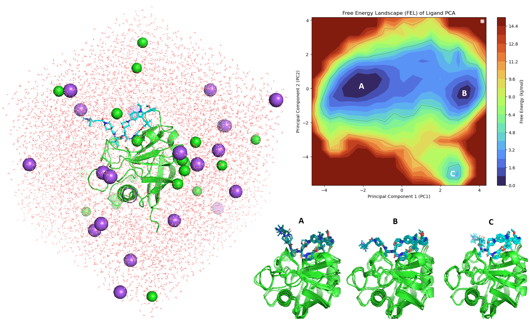
The BPMD analysis confirms the presence of multiple accessible binding modes for the full Elironrasib ligand within the CYPA complex (Figure 15). In contrast, the truncated CYPA binding motif demonstrated high stability under the RMSD perturbation, with only one of the 10 replicas showing a dissociation event (i.e., replica 9). Furthermore, the Potential of Mean Force (PMF) inverted from the bias shows that Elironrasib's binding pose minima are spread across a broad range of the RMSD CV. This result is consistent with the preceding unbiased MD simulations, definitively confirming the high flexibility of Elironrasib when associated solely with CYPA. There appears to be no single, uniquely stable CYPA+Elironrasib neo-interface established prior to KRAS engagement. In my opinion, this binding heterogeneity presents characteristics more typically associated with the transient, multi-state nature of a hetero-bifunctional molecule rather than typically rigid molecular glues such as Immunomodulatory Drugs (IMiDs).
Simulations on Ternary Complex Crystallography and Co-folded Model
To finialise, I did the study by directly comparing the experimentally derived Elironrasib ternary structure (PDB: 9BFX) with the most confident model generated by Boltz-2 in my previous blog. The MD simulation provides a physical framework to estimate complex stability between these two states, offering atomic-level insights into molecular interaction, physiological dynamics, and the mechanism of chemically induced proximity. However, this study first had to overcome a major technical difficulty: How does one accurately parameterise a covalent ligand within a protein complex for simulation?
Building the Force Field for Covalent Ligand within KRAS G12C
Parameterising and simulating proteins that incorporate non-canonical amino acids (ncAAs), including covalently attached ligands, has long been a challenge. Most traditional modelling software packages, such as AMBER and CHARMM, were not fundamentally designed to handle chemical modifications outside of the standard biomolecular space. While platforms like GROMACS and Rosetta offer more flexibility in processing residue topology, they historically demand significant manual effort in pdb/mol file editing as well as cautious parameterisation using QM calculations (very frustrating process I still recall from using Gaussian, Antechamber and tleap for a helical peptidic foldamer project during my PhD).
Thanks to recent advances from the OpenFF team, building force fields for proteins with Post-Translational Modifications (PTMs) is now substantially streamlined via Python code. To parameterise Elironrasib covalently attached to the KRAS G12C mutation, I implemented a workflow structured in three general steps:
Covalent Linkage Definition: The stereochemistry of the new covalent bond was first determined from both the experimental structure and the co-folding model. A Chemical Component Dictionary (CCD) object was created for the new residue type in SMIRNOFF format containing parameters, based on a SMARTS reaction I defined (Figure 16). Then this new modified residue at position 12 was linked within KRAS via the standard peptide backbone bonds.
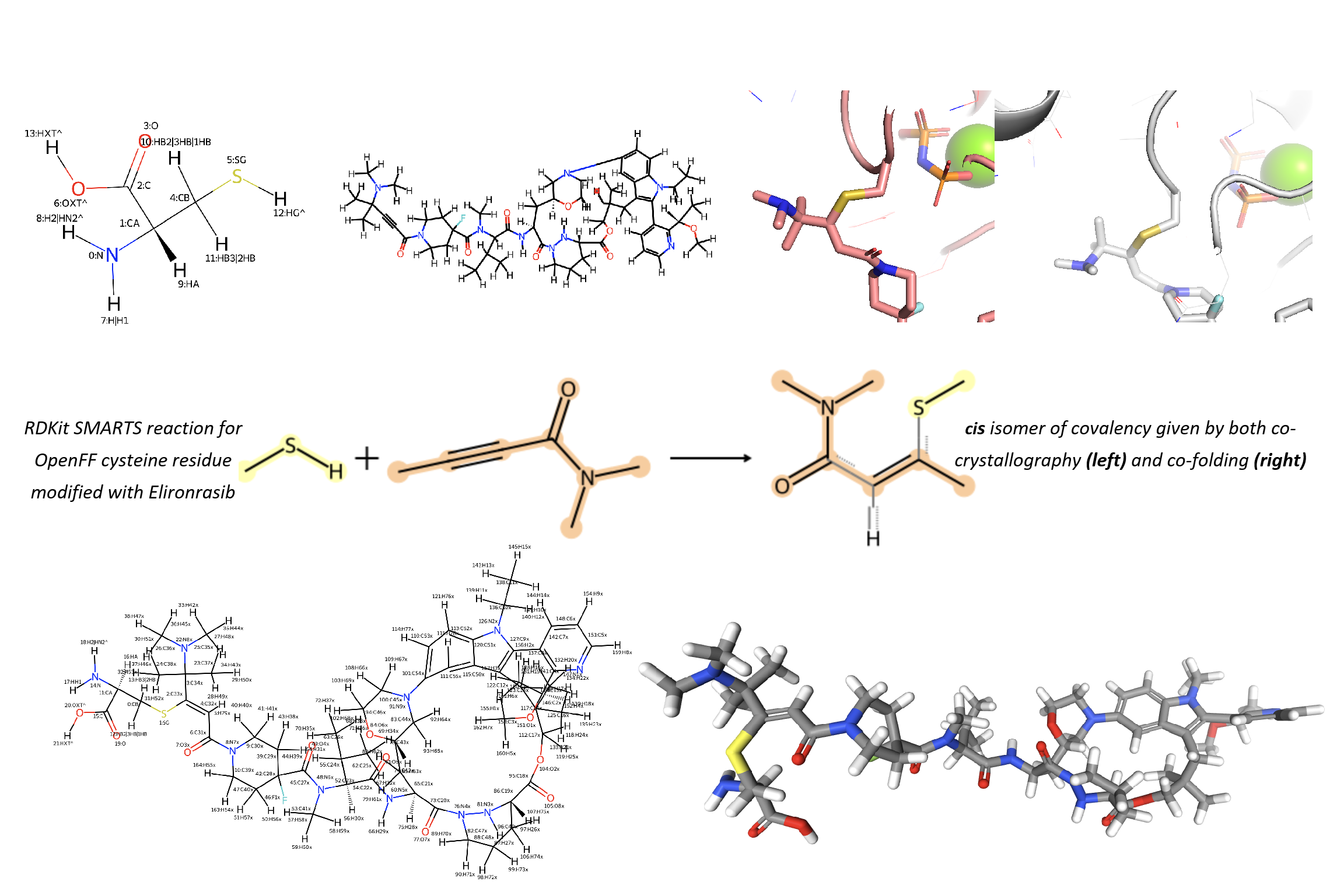
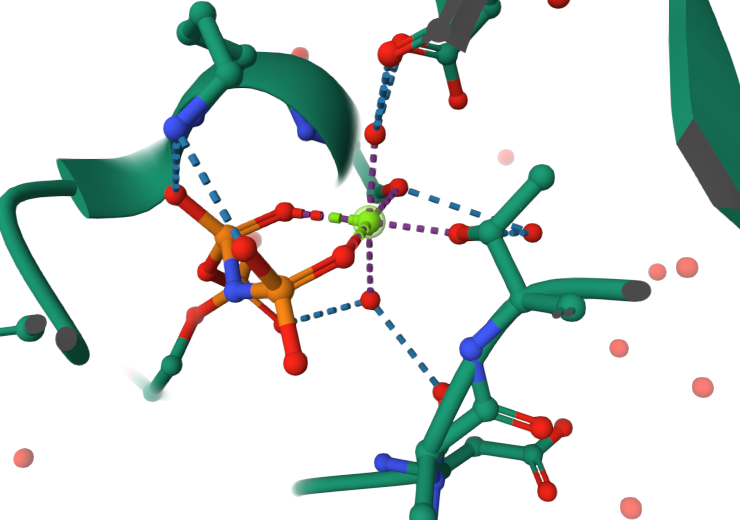
Cofactor Parameterisation: The structure contains the GNP and Mg2+ cofactors. Given the octahedral coordination fitted in the co-crystallography (Figure 17), Magnesium ion, N-phosphates and other coordinating residues like SER18 and THR36 were modified and charged for parameterisation (This might need to proceed with caution since bio-inorganic chemistry falls outside my expertise).
Charge Assignment using NAGL: Both the pdb and sdf structure files were edited to match the topology defined by the customised force field parameters. Atomic charges were then assigned to the entire covalent complex using the graph-based NAGL model (Text 18). This approach efficiently bypasses the BCC or restrained ESP protocols, as a full QM calculation on the entire KRAS-Elironrasib adduct is computationally infeasible on my PC — let alone capturing the necessary conformational dependence of the charges.
# define customised residue database
ligand_resdef = ResidueDefinition.from_molecule(
    molecule=adduct,
    residue_name="LIG",
    linking_bond=PEPTIDE_BOND,
    )
ser_resdef = CCD_RESIDUE_DEFINITION_CACHE["SER"][6].replace(
    residue_name='SEN',
    description='SERINE deprotonated',
    )
thr_resdef = CCD_RESIDUE_DEFINITION_CACHE["THR"][6].replace(
    residue_name='THN',
    description='THREONINE deprotonated',
    )
residue_database_1 = CCD_RESIDUE_DEFINITION_CACHE.with_({"LIG": [ligand_resdef]})
residue_database_2 = residue_database_1.with_({"SEN": [sen_resdef]})
residue_database_3 = residue_database_2.with_({"THN": [thn_resdef]})

# parameterise the edited pdb structure including LIG residue of G12C-Elironrasib adduct
# (all atom names and indices must match the residue database!)
covalent_topology = topology_from_pdb(
    "final_covalent_mod.pdb",
    residue_database=residue_database_3,
)
covalent_topology.box_vectors=None
force_field = ForceField("openff-2.2.1.offxml", "ff14sb_off_impropers_0.0.4.offxml")

# parameterise the Magnesium ion
charge_handler = force_field.get_parameter_handler('LibraryCharges')
mg_charge_params = {
    "smirks": "[#12+2:1]",
    "charge1": 2.0 * unit.elementary_charge
}
charge_handler.add_parameter(mg_charge_params)
vdw_handler = force_field.get_parameter_handler('vdW')
vdw_params = {
    'smirks': '[#12+2:1]',
    'epsilon': 0.07 * unit.kilocalorie_per_mole,
    'sigma': 1.7 * unit.angstrom,
}
vdw_handler.add_parameter(vdw_params)
MG = Molecule.from_pdb_and_smiles('MG.pdb', '[#12+2:1]')
covalent_topology.add_molecule(MG)

# parameterise the GNP cofactor
rdmol = Chem.SDMolSupplier('GNP_H_charged.sdf')[0]
Chem.SanitizeMol(rdmol)
GNP = Molecule.from_rdkit(rdmol, allow_undefined_stereo=True)
GNP.name = "GNP"
for atom in GNP.atoms:
    atom.metadata['residue_name'] = 'GNP'
covalent_topology.add_molecule(GNP)

# solvate the complex model in water (TIP3P) box using OpenFF pablo module
# and assign each molecule with NAGL atomic charges before OpenFF interchange
final_topology = solvate_topology(
    covalent_topology,
    nacl_conc=Quantity(0.1, "mol/L"),
    padding=Quantity(1.0, "nm"),
    box_shape=RHOMBIC_DODECAHEDRON,
)
interchange = parametrize_with_nagl(
    force_field=force_field,
    topology=final_topology,
)
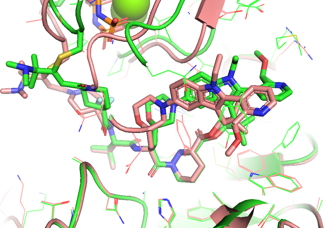
Comparion Between Elironrasib Ternary Complex Crystallography and Co-folding States
Starting from two distinct initial geometries (Figure 19), both 10 ns simulations relaxed each ternary complex into corresponding locally stable states. Geometric analysis indicated that neither trajactory displayed any violent fluctuation, significant conformational change, or complex dissociation. In other words, basic conformational evaluation could not tell us whether the crystallography is 'more correct' or the co-folding model is 'less wrong'...
As a computational chemist with background in small-molecule QM and NMR spectroscopy, my preference is to compare the potential energies directly across different states. However, obtaining meaningful free energy differences (∆G) in biomolecular statistical mechanics is difficult. This is due to the varying size of explicit water molecules necessary in bulk environment and the distinct complex conformations, which would necessitate extensive enhanced sampling (Umbrella Sampling, Weighted Ensemble, MSMs etc.) to explore possible transition pathway(s) on the force-field level landscape. This differs significantly from methods like FEP/TI transformation, which typically need to handle very tiny chemical change within a similar binding mode.
Hence I pursued the following three approaches for feasible comparison:
End-state MMPBSA Calculations: This method approximates explicit solvent effects using the Poisson-Boltzmann surface area. Unfortunately, the AMBER module I attempted to use does not technically support customised force-field topologies involving both the covalent ligand and the metal cofactor. While Schrödinger’s toolkit like ProteinPrep and Prime are able to handle this, I have elected to avoid commercial software in this personal blog.
Solute RMSD-Based Targeted MD: After equalising the two systems (e.g., water count in the PBC box) and aligning them by the CYPA domain, I applied a harmonic constraint (OpenMM constant force 1000.0 kJ/mol/nm^-2) to steer the KRAS position in the complex from the co-folding model toward the crystallography pose. However, the kinetic barrier associated with the Elironrasib atropisomerism prevented successful crossing through such smooth SMD protocol, thereby disabling a full recovery of the bias for relative PMF estimation.
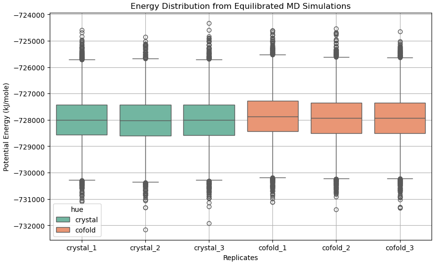
Comparison of Total Potential Energies: Utilising the same system equalisation and alignment as the previous attempt, I compared the distribution of total potential energies once the systems relaxed to equilibrium. Across all three 50 ns production replicates (Figure 20), the ensemble corresponding to the relaxed crystallography state demonstrated lower mean/median/mode potential energy scores than those simulated from the most confident co-folding model.
Waters - A Possible ‘Rationalisation’ from the Perspective of Biophysics
In my opinion, computational chemistry fundamentally provides a result of 'yes or no'. This physics-based science is not inherently designed to answer medicinal chemistry questions such as 'why or why not', a task that requires critical human interpretation. This gap only widens when dealing with the 'black box' nature of AI driven by data. Although these 'why' questions are daily requests from our industry colleagues about understanding SAR, I consciously avoid getting into the weeds of detailed model explanations and instead focus on supplying clear, testable hypothesis which could guide the drug design effectively. Herein, I hypothesise that the poor co-folding prediction for Elironrasib ternary complex is directly attributable to the model's failure to explicitly account for water solvation effects.
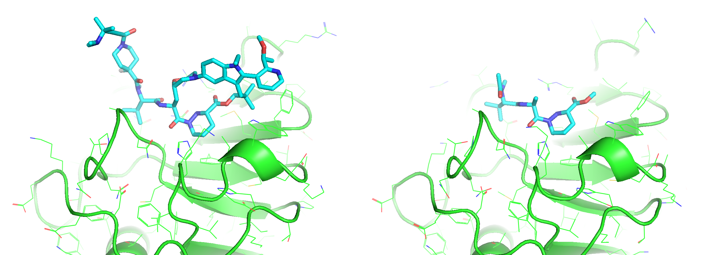
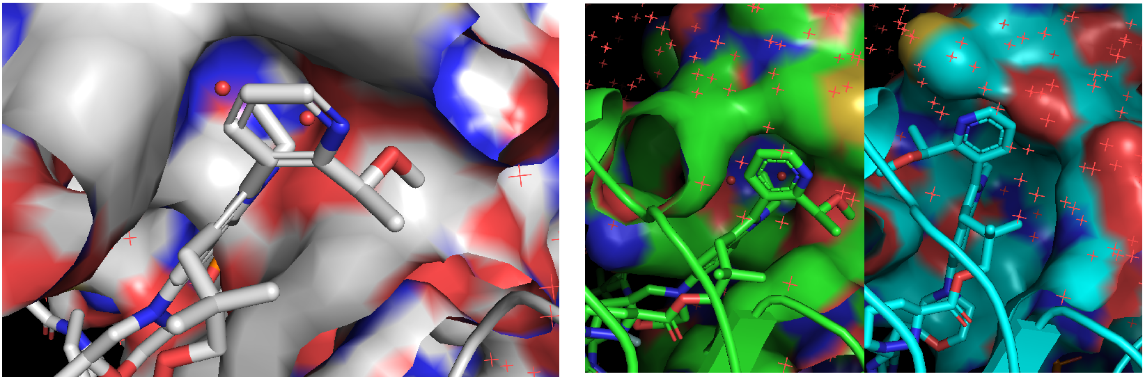
For both isomorphous ternary complexes packed in the crystallography (PDB: 9BFX), the correct antropisomer of Elironrasib could accommodate over two buried structural waters on the KRAS surface (Figure 21 left). These waters effectively lock the complex and help form perfect complementarity, significantly contributing to the Buried Surface Area (BSA) in the complex as I mentioned in the last blog. This observation was confirmed by most snapshots clustered from the long MD relaxation (Figure 21 right), even though all waters were initially inserted randomly. The crystallography water map was successfully refined by the simulation (green), whereas the AI co-folded model resulted in significantly more disordered waters around the interface (blue) that indicate poor proximity and stability induced by the wrong atropisomer of ligand.
In several short MD tests beforehand, when waters failed to position correctly like those packed in the crystallography, the corresponding systems' potential energies were at a similar high level to those simulated from the co-folded model containing the wrong ligand atropisomer. While other physical methods, such as Grand Canonical Monte Carlo (GCMC), might offer a better approach to compare these systems, these MD simulations at least demonstrates:
1. The importance of water molecules for ternary complex stability.
2. A piece of missing puzzle for most promising AI co-folding predictions currently applied to protein-ligand complexes.
Outlook
In this blog, I have tried to estimate some foundation ML models and AI co-folding predictions in details based on my background in molecular physics. For computational chemistry and CADD more practically, there are few more important topics - QSAR and chemical generation. These fields have traditionally and currently been sustained by robust cheminformatics methodologies. However, the industry is witnessing an explosive growth of large and generative AI models being deployed for specific tasks, rapidly reshaping R&D landscape. In my next blog (which I hope to complete in the new year after Christmas), I will test and compare some of these cutting-edge generative chemistry models, potentially focusing on applications within the Targeted Protein Degradation (TPD) and/or covalent drug discovery fields where I have sufficient experience. Please keep an eye out for this continuation!
Data and Code Availability
Acknowledgement
This personal blog post was made possible with excellent open-source, academic, or non-commercial-use software, models, toolkits and platforms below under corresponding licenses:
OpenMM - Major molecular simulation toolkit, optimised for high-performance GPU computing using openmm. The REST simulation was performed with openmmtools and the ML/MM simulation followed the tutorial in openmm_workshops.
OpenFF - Provides modern SAGE force field parameterisation using openff-toolkit. The covalent topology was built by the package openff-pablo. The graph-based charge model was from openmm-nagl.
ORCA - General-purpose quantum chemistry software package orca for cutting-edge DFT calculations fast and accurately.
XTB - Semi-empirical quantum mechanics program xtb developed by the Grimme group, used for geometry optimisation on samples from molecular mechanics.
GROMACS - High-performance GPU/MPI accelerated molecular dynamics simulation engine gromacs, running and analysing molecular mechanics systems built from OpenMM and OpenFF.
AmberTools - Suite of programs ambertools for general AMBER force fields setup and parameterisation.
MDTraj - Molecular dynamics trajectories analysis library mdtraj.
OpenBPMD - Implementation of binding pose metadynamics program openbpmd from the Gervasio group, built on OpenMM platform.
pkasolver - Machine learning model toolkit pkasolver for predicting pKa values of small molecules using graph neural networks.
TorchANI - ANI-style neural network interatomic potential library torchani, built with PyTorch platform.
MACE - Seires of machine learning interatomic potentials mace, with advanced graph architecture based on PyTorch.
Meta FAIR Chemistry - Library of machine learning methods for chemistry by Meta fairchem, including UMA models and OMol datasets used for atomic NNPs.
Google Gemini - Large Language Model Gemini by google used to advise research workflow, provide coding/debugging assistance and supply writing refinement.
Disclaimer
The entirety of the content, methodologies, analyses, and conclusions presented in this personal blog post are solely the contribution of myself as the author, and are based exclusively on open-source, non-commercial-use software and publicly available data. This work is intended purely for academic and educational use and is not related to, reflective of, or affiliated with the work, practices, or proprietary information of any of my current or previous employers.