
Some ‘Learning’ in Cheminformatics, QSAR and Generative AI
Published:
Introduction
In 2025, I published two posts exploring molecular modeling through AI co-folding and physics-based simulations for Structure-Based Drug Discovery (SBDD), drawing on my background in physical organic chemistry and biophysics. However, some pillars of modern computational drug discovery - Cheminformatics and Machine Learning (ML) - have yet to be discussed here. During my time in the industry, these are the fields where I have experienced the most significant professional growth.
In this post, I will share insights from my journey transitioning between the roles of a cheminformatician and an ML engineer within the biotech ecosystem. To demonstrate the real-world application of data science in drug discovery, I will present a virtual screening (VS) workflow targeting the Cereblon (CRBN) chemical space for covalent drug discovery (Figure 1). We will walk through a rigorous pipeline: from chemical database mining and library enumeration to molecular docking, QSAR modelling, and AI-driven generation - all guided by the rational constraints of organic and medicinal chemistry.

Study Outlines
Data Inspection & Curation - Analysing the chemical space of CRBN-based binders and degraders using both open-source and commercial databases.
Chemical Library Enrichment - Using traditional cheminformatics and Quantum Mechanics (QM) approaches to generate synthetic data, specifically addressing regions of insufficient chemical space for the coverage of covalent modalities.
Physical Validation for VS - Implementing shape-constrained molecular docking to screen large-scale chemical libraries, refining the candidate space based on realistic binding poses and steric complementarity.
QSAR Modelling & Hit Identification - Developing classical ML models (SVM, tree models) and Graph Neural Networks (GNNs) to classify, regress and prioritise the chemical space of interest (CRBN-based covalent modulators).
Generative AI & Rational Optimisation - Evaluating industry-standard generative models, including the smilesRNN module from the MorganCThomas/Nxera team and the REINVENT4 reinforcement learning platform developed by AstraZeneca, together with post-processing by alert filtering, descriptor scoring, and transferred QSAR models for the final selection in drug design.
Chemical Database Search and Processing
The public domain offers a vast array of chemical databases — including PubChem, ChEMBL, ZINC, and Enamine — each serving distinct research purposes. As a computational medicinal chemist actively supporting Targeted Protein Degradation (TPD) pipelines, I have found BindingDB and MolecularGlueDB particularly effective for capturing academic datasets.
In an industrial setting, we also place a high premium on the latest competitive intelligence, often found in patent literature. Extracting, annotating, and structuralising this "dark data" requires significant effort... Fortunately, AI-powered tools like DECIMER (used later in this workflow) have streamlined the translation of chemical images into machine-readable formats. Furthermore, efficient drug design necessitates libraries built upon synthetically feasible building blocks. Chemical suppliers such as Enamine provide some useful catalogs that allow us to tailor our search criteria to the specific synthetic constraints of a project.
While sourcing data is foundational, the engineering approach used to process them is often the differentiator in a project's success. For professional cheminformatics workflows, I prefer KNIME pipeline as learnt on the job. This GUI-based platform is exceptionally powerful for manipulating and visualising tabular data (such as CSV or SD files with chemical structure) through sequential nodes. Honestly KNIME has saved me countless hours typically spent on boilerplate data engineering with Python (including RDKit, Pandas, and NumPy modules). While LLM-driven AI agents are evolving, I remain cautious about fully delegating these tasks to them. I believe data processing in chemistry still needs deep domain expertise and human-level ability to perform real-time monitoring and debugging, which also ensure integrity and accountability as required in industry.
Open-source Curation and Data Imbalance
The Figure 2 illustrates the KNIME workflow I developed to aggregate and process CRBN chemical space data from BindingDB and MolecularGlueDB. Beyond generating the final dataset in SDF format, the pipeline extracts available PDB structural metadata for downstream structural analysis. To assess the chemical diversity, I employed t-distributed Stochastic Neighbor Embedding (t-SNE), a dimensionality reduction technique used here to project the chemical space based on molecular fingerprints and Tanimoto similarity.
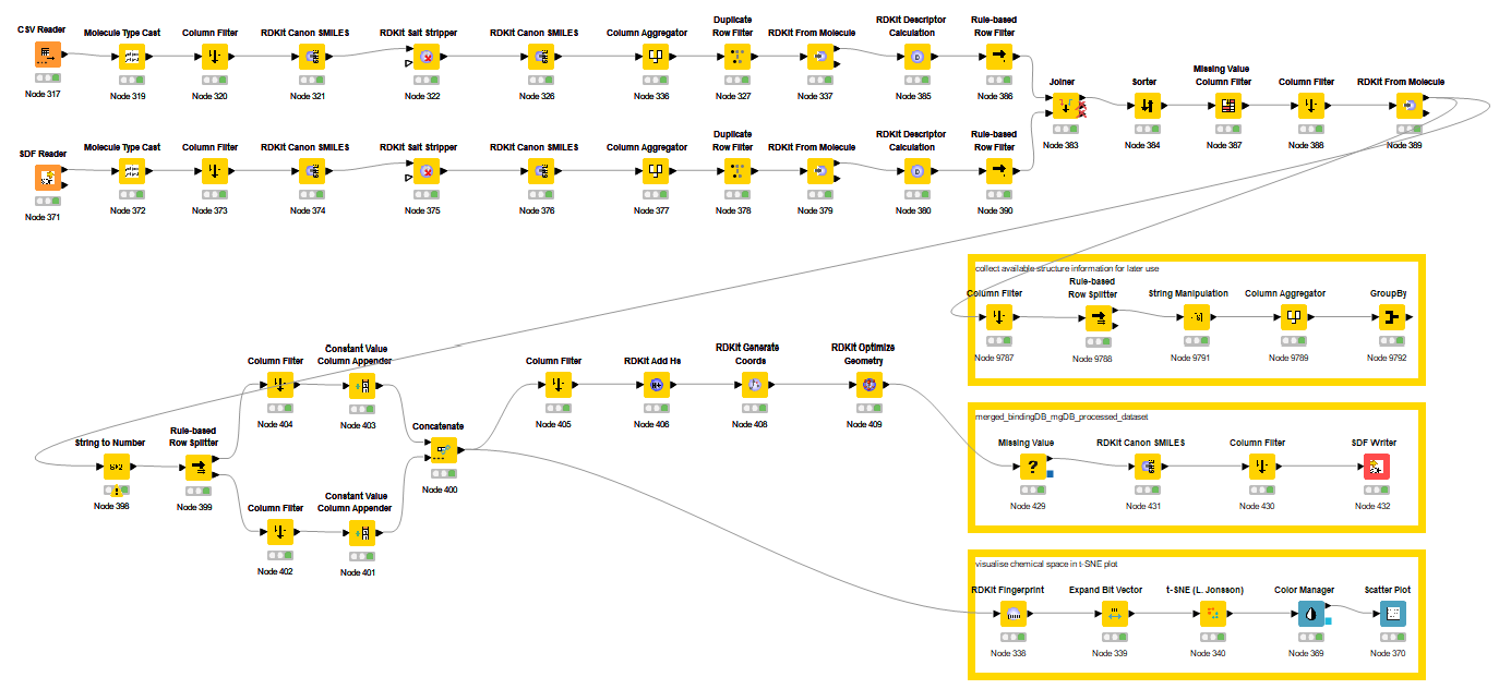
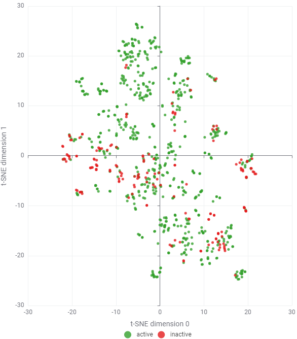
Since high-molecular-weight PROTACs (> 600 Da) were filtered out, the remaining dataset consists of a few hundred small-molecule CRBN binders and glues. Given this relatively small scale, I utilised 1024-bit Morgan fingerprints (radius = 2, chirality ignored) without significant concern for bit collisions. The most labor-intensive step, however, remains the manual classification of "active" versus "inactive" sets. This requires a detailed review of diverse data sources, varying biophysical or cellular assay conditions, and vague thresholding (e.g., **) — all of which demand cautious, expert-led curation. As shown in Figure 3, there is a major challenge obviously: An overwhelming prevalence of "active" compounds relative to "inactive" labels. This reflects the publication bias in open databases, where academic research naturally prioritises and reports successful positive results.
In industry, the situation is usually opposed. In the Design-Make-Test-Analyze (DMTA) cycle, we typically generate far more negative data than positive hits. Relying solely on these limited and imbalanced public datasets for QSAR modeling is often not productive. To build a robust predictive model, we must look beyond these biased activity labels and seek opportunities in broader, unlabelled chemical libraries or through data augmentation.
Commercial Database & Cheminformatics Analysis
Recently, Enamine released several targeted libraries focused on CRBN molecular glues (the link in reference). I found these datasets are highly informative and chemically diverse, spanning a range of scaffolds from classic IMiDs to newer derivatives such as Phenyl Amino Glutarimides (PAG), Phenyl Dihydrouracils (PD), Phenyl Glutarimides (PG), Acylated Amino Glutarimides (AAG), and Avadomide.
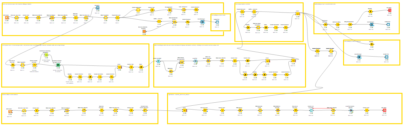
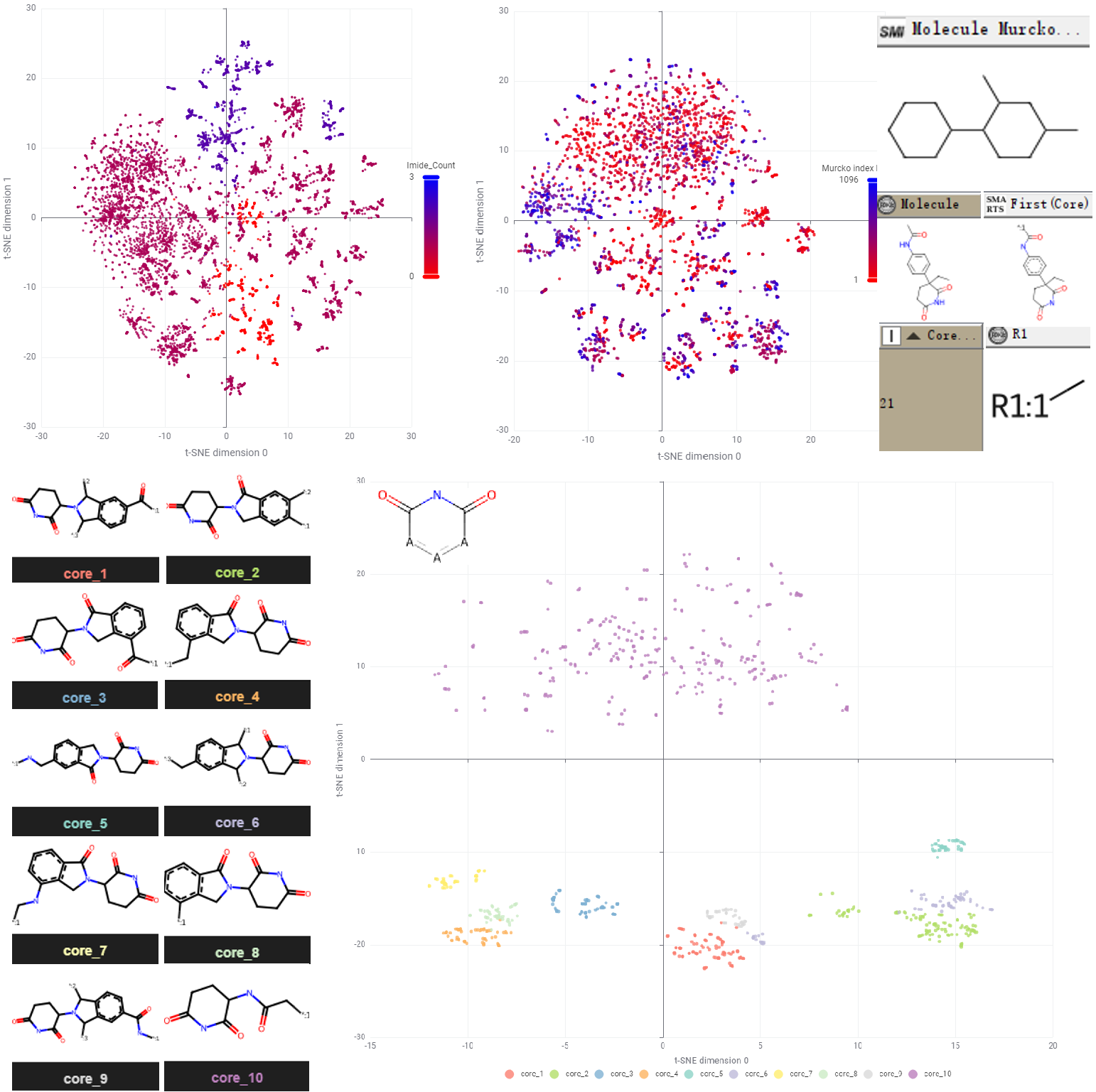
Using a custom KNIME workflow (Figure 4, upper), I analysed this chemical space at multiple levels. At the molecular level, the dataset contains over 3,000 unique canonical SMILES strings (processed by stripping stereochemical tokens like '@' to simplify initial analysis). As expected, the vast majority of these molecules contain at least one cyclic imide substructure, acting as the essential pharmacophore for CRBN binding (Figure 4, lower).
However, raw t-SNE visualisations at the molecular level can appear "fuzzy" due to the high density of similar scaffolds or near-duplicate analogs — a problem that alternative algorithms like UMAP also struggled to resolve. To achieve a more distinct and interpretable visualisation, I abstracted the molecules to their Bemis-Murcko scaffolds (retaining only the union of ring systems and linkers) and performed Maximum Common Substructure (MCS) decomposition.
This hierarchical mapping revealed that while the majority of core scaffolds are rooted in the IMiD class, the merged dataset successfully captures modern chemical matters. For instance, cores 10 and 21 respectively represent the more recently developed PAG and PG scaffolds (Figure 4, lower). This structural decomposition allows us to better navigate the diversity of the library and identify gaps for potential expansion.
Addressing the Covalent Modality Gap
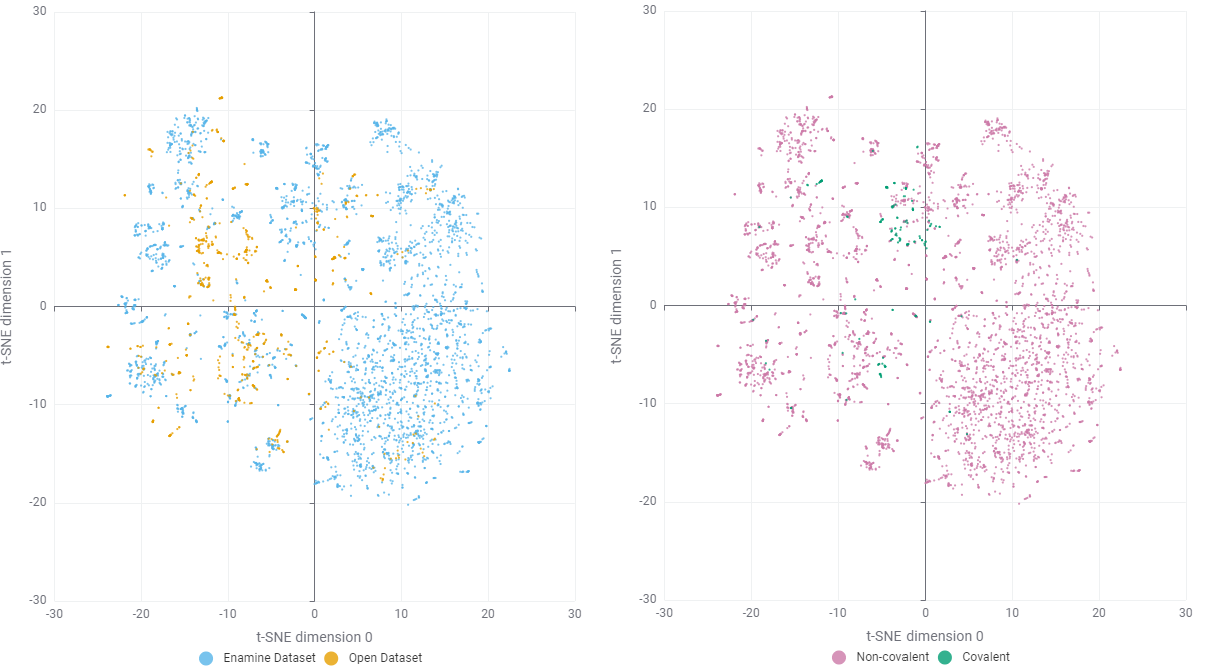
By merging the curated public dataset with the Enamine library, I was able to significantly enrich the available chemical space (Figure 5). There is minimal overlap between the two: This is likely because commercial suppliers prioritise novel, synthetically accessible analogs rather than simply replicating previously reported active substances. Despite this expansion, a critical gap remains: Covalent CRBN binders and their corresponding degraders are still under-represented, accounting for only ~150 entries out of the 4500 records in the final library.
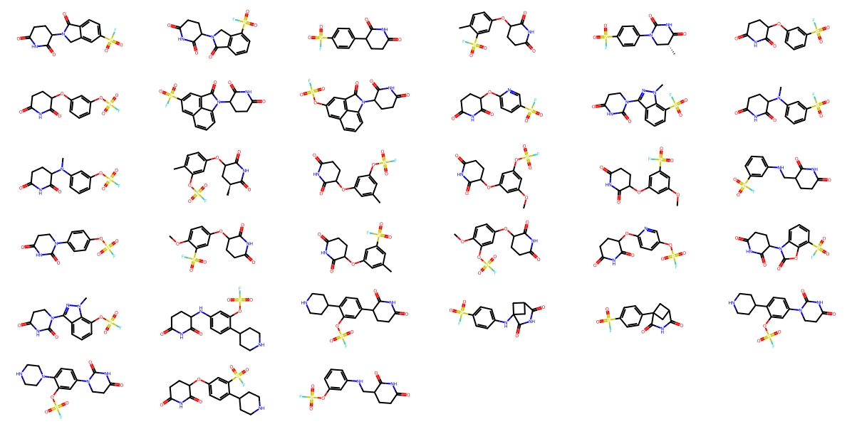
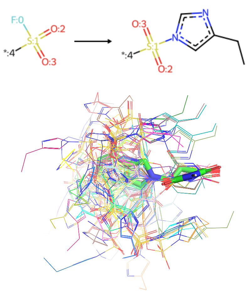
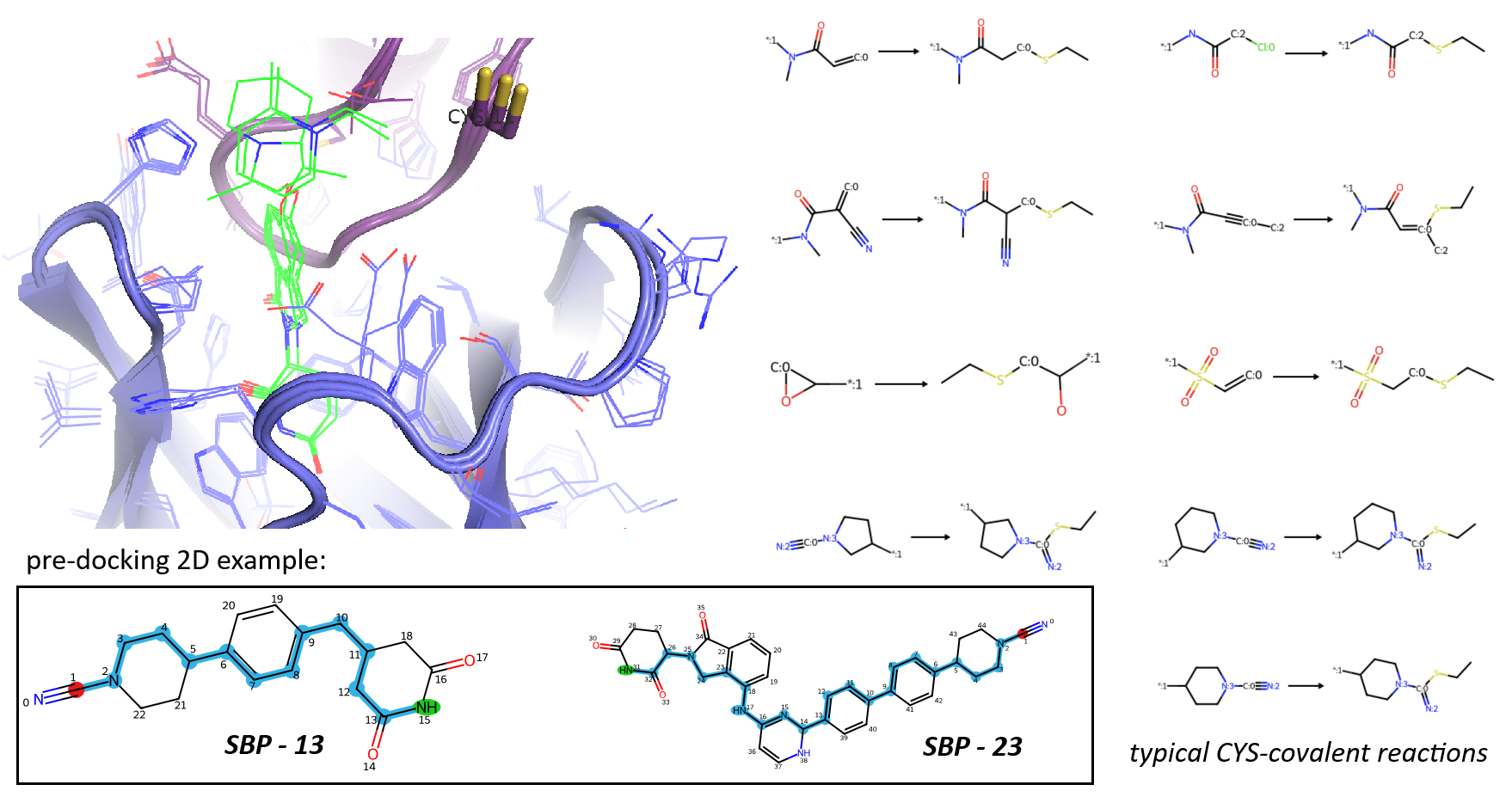
To address this sparsity, I conducted a targeted literature and patent search, focusing on recent works from the Lyn Jones group in Dana-Farber (the DOI in reference) and a recent C4 Therapeutics patent (WO2025/096856A1). This yielded approximately 30 additional covalent CRBN binders not present in the initial databases (Figure 6). Based on the reported mechanism, most of these ligands function as reversible-covalent binders that target HIS-353 through a sulfonyl fluoride warhead (as shown in the left, Figure 1).
From my perspective as drug designer in TPD industry, the potential for covalent modalities in CRBN-dependent degradation is far broader than what is currently documented. Recent structural data and pipelines from AstraZeneca, BMS, MonteRosa and Novartis suggest several untapped opportunities:
- The IKZF2 neosubstrate features a HIS-6 residue on its beta-sheet near the G-loop (middle, Figure 1).
- The WIZ neosubstrate also contains a CYS-11 residue positioned near the IMiD-binding pocket on CRBN (right, Figure 1).
Both residues present strategic handles for covalent engagement. The challenge now lies in how to “invent” and explore this hypothetical chemical space in silico to target these specific residues.
Synthetic Data Generation via Classic Cheminformatics
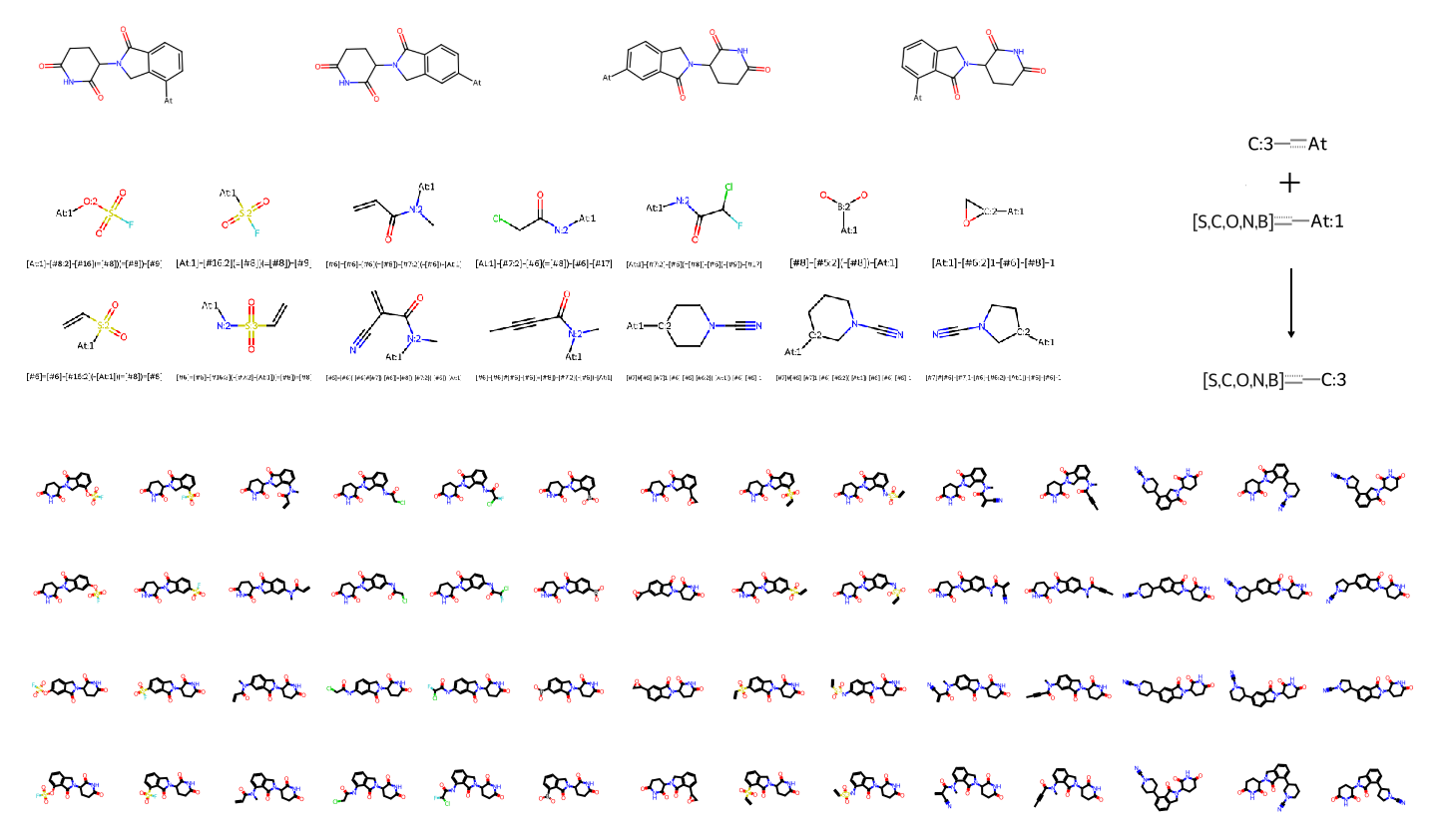
In cheminformatics, one of the most robust methods for library enumeration is the use of virtual reactions between building blocks (synthons). This approach ensures that the resulting "drug-like" molecules are synthetically accessible for wet-lab validation. Given that most IMiD and glutarimide derivatives in my current dataset feature phenyl or/and other aromatic systems, I utilised a C-H activation strategy to append covalent warheads virtually.
For this rapid enrichment, I defined a two-component Reaction SMARTS using RDKit to functionalise sp2-hybridised [c;H1] atoms on each candidate in the dataset (Figure 7). A suite of 14 warheads commonly employed in covalent drug discovery were curated for targeting proximal cysteine or histidine residues. This strategy successfully transformed non-covalent precursors into a vast, covalent-focused chemical space.
To ensure the robustness and quality of the generated library, I implemented several critical post-processing steps:
Deprotection: Before the aromatic C-H activation, I applied other SMARTS-based transformations to remove common protecting groups (e.g., converting carbamates to amines, ester hydrolysis, and hydroxyl deprotections).
Scaffold Simplification: Prior to covalent transformation, I also abstracted the diverse structures into their Bemis-Murcko scaffolds to simplify the hit library, reducing the starting pool from approximately 4000 to 2500 unique frameworks.
Quality Control: After enumeration, I verified the presence of the essential imide pharmacophore and filtered out undesired substructures using a modified PAINS list - Carefully excluding the phthalimide core and the intended reactive warheads from the ‘bad’ SMARTS filter.
During this process, I leveraged AI agents like Gemini and Claude via my Copilot Pro account to assist with coding. While these LLMs generated each individual RDKit function perfectly they struggled with the "big picture" logic required for complex database workflows. Without iterative, human-led direction (through structured markdown protocols and specific prompts), these agents sometimes failed to clean protective groups or just generated invalid SMARTS variables. This underscores a current truth for industry-level applications: While LLMs are powerful coding assistants, we still require chemistry-specialised language models to fully automate the digital stage of drug discovery with scientific logic.
Anyway, this cheminformatics workflow yielded 137673 potential covalent CRBN candidates (all with MW < 600 Da). Within this set, 19678 entries contain sulfonyl fluoride or fluorosulfate groups for targeting histidine, while the remainder are supposed for cysteine reactivity. With a redundant chemical space at the moment, I decided to use physics-based refinement in next stage to confidently identify high-priority hits.
Covalent Docking with Structural Constraints
To screen the ~140000 candidates generated from our enumeration, I employed molecular docking guided by high-resolution structural data rather than co-folding model. A query of the RCSB PDB reveals that most available structures represent the "closed" (active) state of CRBN, which is the conformation required for neosubstrate degradation. These include both the isoform 4 (UniProt A4TVL0) and standard human (UniProt Q96SW2) sequences. Their experimental structures are essential for prioritising chemical space for covalent modulators, molecular glues, and PROTACs.
Ensuring Reliability in Docking Models
For the initial ensemble docking validation, I selected three high-resolution crystal structures of human CRBN in the closed binary state: 4TZ4, 5V3O, and 8OJH (Figure 8). These structures show highly conserved IMiD-binding sites. By aligning these models, I established a consistent set of structural constraints to "lock" the chemical space and ensure our virtual screening remains biologically relevant.
Preparing Ligand before Docking
For the covalent docking workflow, I utilised the flexible sidechain mode of AutoDock4 (AD4). This method involves masking the target covalent residue's atom types and charges in the PDBQT grid map, while the ligand-adduct is "anchored" to the protein backbone at the Ca position. To prepare these conjugates, I defined a SMARTS-based transformation to create the object of ligand-sidechain adduct in 2D (Figure 9).
Furthermore, I performed a two-step conformer preparation:
- Conformational Sampling: Initial 3D rotamers were generated using the ETKDG method followed by MMFF minimisation.
- Pharmacophore Alignment: A shape-alignment filter was applied, selecting only those conformers where the cyclic imide pharmacophore maintained an RMSD < 2 Å relative to the bioactive glutarimide pose.
Through providing a pre-aligned "bioactive-like" starting conformation for the glutarimide ring, the AD4 Genetic Algorithm only needs to explore the remaining freely rotatable torsions under translational and rotational transformations, significantly improving the efficiency of the search within the fixed grid.
Overcoming Docking Pose Drift with Custom Constraints
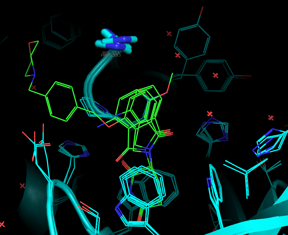
A common challenge in virtual screening is "pose drift", where ligands dock into peripheral cavities rather than the intended pocket. Even with a defined grid box (20-30 Å), we often observe geometry clusters where the ligand deviates from the reference IMiD coordinates. For example, in one test case below, 4 out of 5 docking clusters occupied sites distal to the IMiD pocket (Video 10).
Vedio 10. A covalent CRBN docking example showing diverse binding modes generated from AD4 algorithm and scoring functions, which must require further filtration and selection.While commercial software like Schrödinger Glide offers built-in constrained docking by core or/and shape with a reference ligand, I developed a custom solution by instructing my AI agent to write an RDKit-based post-docking filter (Text 11). This function calculates the MCS-based RMSD of the glutarimide core against the crystal ligand pose. Since the docking was performed in a fixed coordinate system, no further alignment is required - We can simply filter for poses that maintain the essential binding geometry of the imide headgroup.
def get_mcs_rmsd(query_sdf_path, ref_sdf_path, aligned_sdf_path, aligned=False, cutoff=2.0):

    confs = []
    with Chem.SDMolSupplier(query_sdf_path, removeHs=True, sanitize=True) as suppl_query:
        for conf in suppl_query:
            if conf is None: continue
            confs.append(conf)

    with Chem.SDMolSupplier(ref_sdf_path, removeHs=True, sanitize=True) as suppl_ref:
        ref_mol = suppl_ref[0]

    mcs = rdFMCS.FindMCS([confs[0], ref_mol], completeRingsOnly=True, ringMatchesRingOnly=False)
    patt = Chem.MolFromSmarts(mcs.smartsString)

    #check patt contains imide
    imide_smarts = "[!#1]1(-[#6]-[#6]-[#6](-[#7]-[#6]-1=[#8])=[#8])-[!#1]"
    imide_mol = Chem.MolFromSmarts(imide_smarts)
    if not patt.HasSubstructMatch(imide_mol):
        print("Warning: auto MCS does not contain a cyclic imide group, use defined cyclic imide as MCS instead")
        patt = imide_mol
    refMatch = ref_mol.GetSubstructMatch(patt)

    rms_min = None
    best_conf_id = None
    for i, conf in enumerate(confs):
        mv = conf.GetSubstructMatch(patt)
        if aligned == False:
            rms = AllChem.CalcRMS(conf, ref_mol, map=[list(zip(mv, refMatch))])
        else:
            rms = AllChem.AlignMol(conf, ref_mol, atomMap=list(zip(mv, refMatch)))
        if (rms_min is None) or (rms < rms_min):
            rms_min = rms
            best_conf_id = i

    if rms_min <= cutoff:
        with Chem.SDWriter(aligned_sdf_path) as writer:
            conf_with_hs = Chem.AddHs(confs[best_conf_id], addCoords=True)
            conf_with_hs.SetProp("_RMSD_MCS_to_ref", str(rms_min))
            writer.write(conf_with_hs)
        print(f"{aligned_sdf_path} is best valid conformation ID: {best_conf_id} with MCS RMSD: {rms_min} to {ref_sdf_path}")
        return best_conf_id, rms_min
    else:
        print(f"No valid conformation found with MCS RMSD <= {cutoff} A for {query_sdf_path} against {ref_sdf_path}")

        return None, None
Virtual Screening Results
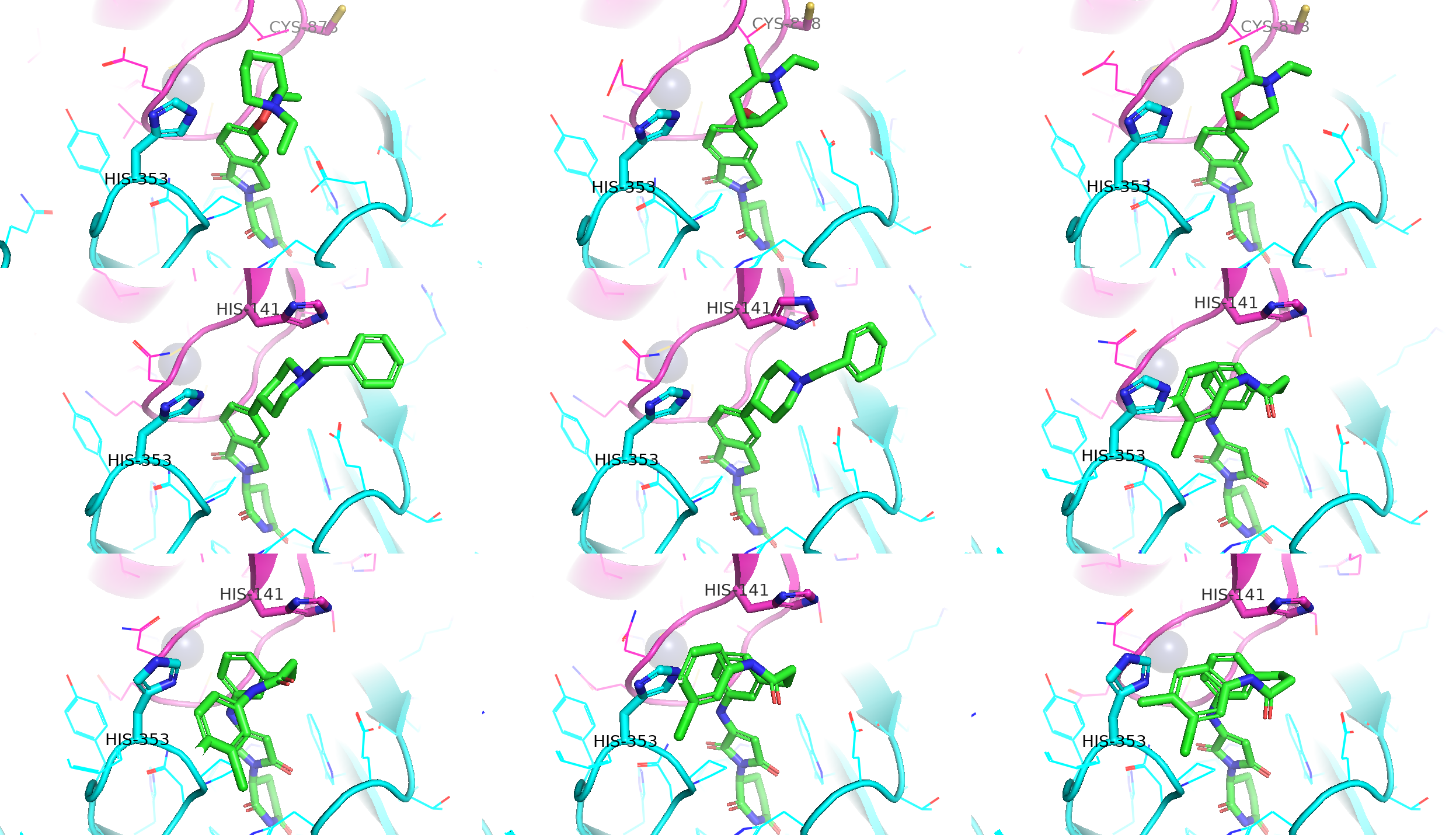
Following several days of intensive computation locally using the docking strategies described above, I successfully refined the in silico chemical space for covalent CRBN binders and degraders targeting IKZF2 and WIZ. The virtual screening for covalent ligands in the binary and IKZF2 ternary complexes was relatively straightforward, as two target histidines are in close proximity to the IMiD binding site near the G-loop (middle and lower rows, Figure 12). In contrast, CYS-11 in the WIZ neosubstrate is more distal from the glutarimide-binding pocket (upper row, Figure 12). This structural gap necessitates "PROTAC-like" bifunctional scaffolds to bridge the distance and ensure effective proximity for covalent engagement.
Covalent CRBN Binders and IKZF2 Degraders
For the covalent CRBN modulators in binary system, 36554 valid poses passed the initial docking and pharmacophore filter (Video 13). To streamline downstream QSAR and generative AI studies, these 3D poses were converted back to 2D canonical SMILES. I also decided to remove stereochemical labels at this stage, as the chiral center at the C3 position of the glutarimide ring is known to racemise rapidly in vivo.
Video 13. All ensemble docking poses that are selected to match the Glutarimide pharacophore in reference ligands from binary co-crystallography (4TZ4, 5V3O and 8OJH).The resulting 14042 unique molecules were filtered using three empirical criteria to ensure drug-likeness and minimise docking artifacts:
- Binding Score (AD4 covalent mode): < -10 kcal/mol to ensure the basic proximity needed
- Molecular Weight (MW): < 500 Da to mitigate the inherent bias of docking algorithms toward larger molecules
- Rotatable Bond Count (nRotB): < 7 to keep conformational stability while limit entropic penalties
These rigorous filters refined the library from over 14000 candidates to a high-priority set of approximately 1500 compounds (Figure 14). 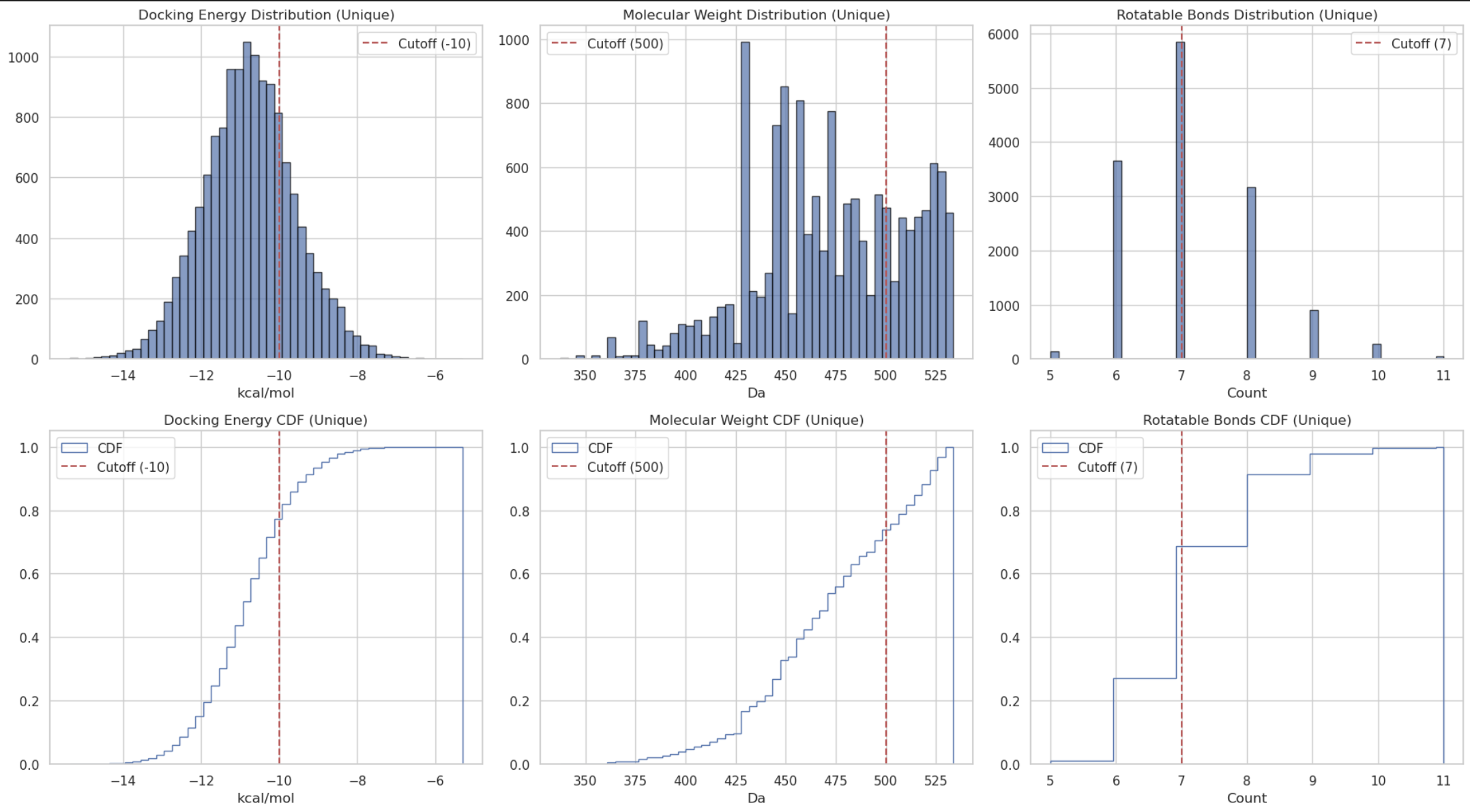
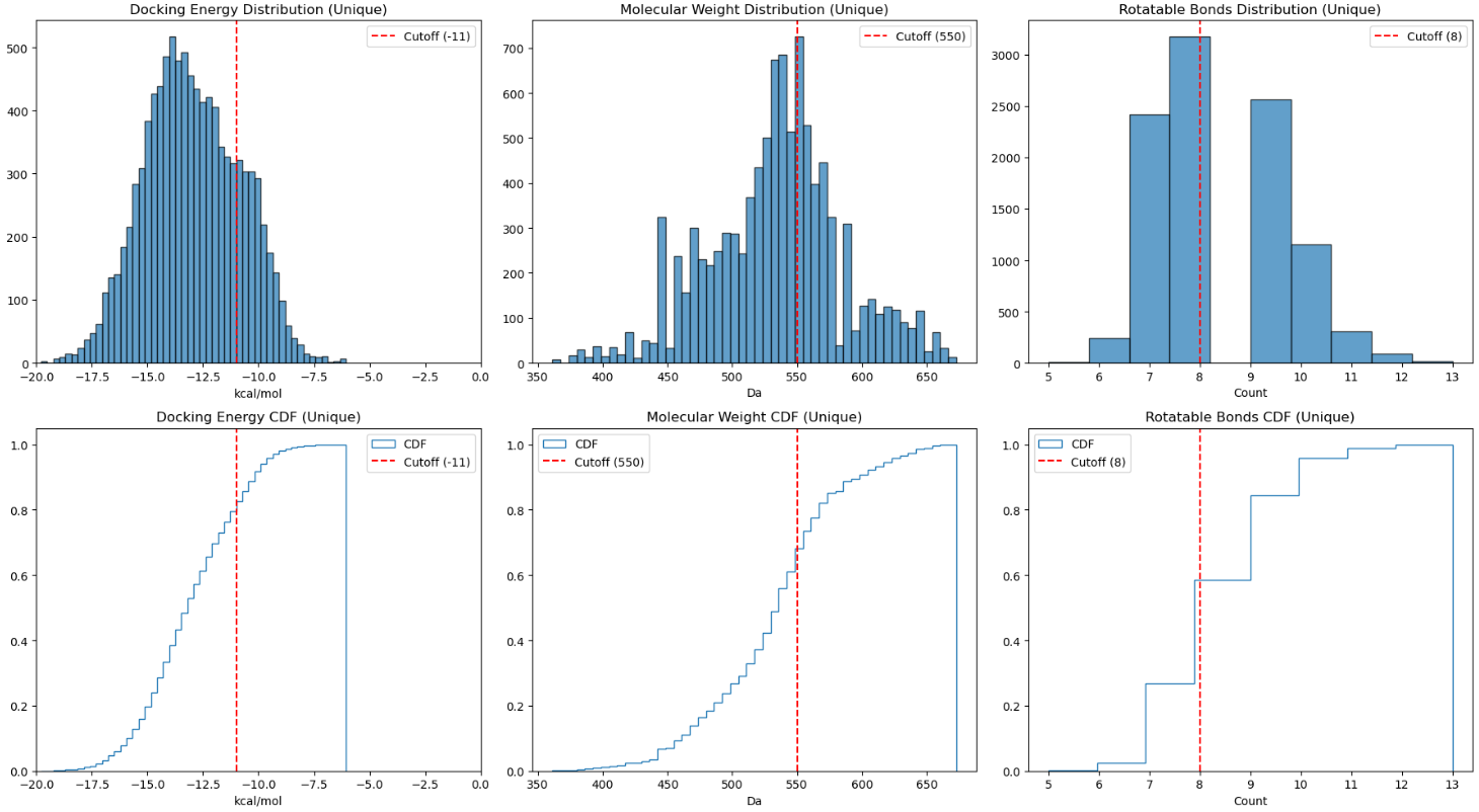
For the IKZF2 covalent MG degraders, I adjusted the thresholds to reflect the increased complexity of the ternary interface: I loosened the MW and nRotB limits (< 550 Da and < 8) but tightened the binding score cutoff (< -11 kcal/mol). This ensured high complementarity within the ternary complex (Video 15 & Figure 16). Approximately 1000 entries were prioritised therefore, with several candidates showing excellent shape complementarity to the exposed aromatic pharmacophores in reference, providing strong structural hypotheses for further medicinal chemistry optimisation.
Video 15. All ensemble docking poses that are selected to match the Glutarimide pharacophore in reference ligands from IKZF2 ternary complexes (7U8F and 7LPS).
Covalent WIZ Degraders
Targeting CYS-11 in the CRBN-WIZ complex presented a greater challenge - Cysteine residues typically require different warheads than histidine, and as noted, the residue is located further from the binding interface. To focus the library as suggested by Gemini, I calculated the Shortest Bonding Pathlength (SBP), the number of bonds on the 2D graph from the imide nitrogen to the electrophilic carbon, using a custom RDKit function. I restricted the library to precursors each with SBP >= 13 to ensure the linker was long enough to reach the target residue (Figure 17).
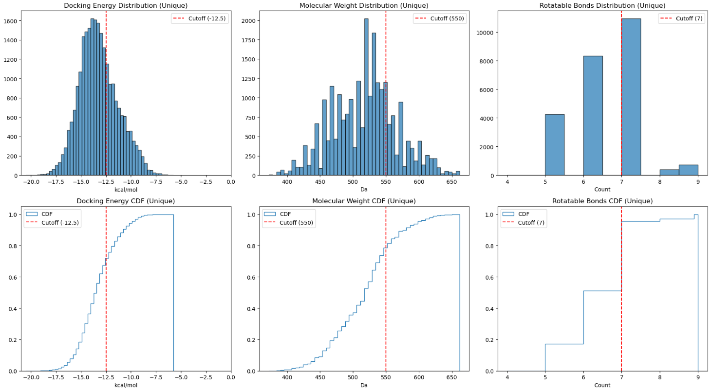
Covalent docking against WIZ yielded several promising drug-like hits (Video 18). For this set, I tightened both the docking score (< -12.5 kcal/mol) and nRotB (< 7) to prioritise PROTAC-like molecules with high "cooperativity" and low internal strain (Figure 19). Interestingly, the top-scoring candidates predominantly featured cyanamide warheads, with fewer types of Michael acceptor. Many of these "winners" adopted L-shaped conformations, perfectly complementing the CRBN-WIZ interface. Again these designs are attached in my repository for any potential development of interest.
Video 18. All ensemble docking poses that are selected to match the glutarimide pharacophore in reference ligands from WIZ ternary complexes (8TZX and 9DJX).
QSAR Modelling
Following virtual screening results above, I merged all prioritised covalent candidates with the original non-covalent CRBN binder pool to create an enriched, multi-modality database. To ensure high-quality leads, I applied a final filter using the Quantitative Estimate of Drug-likeness (QED) score, setting a threshold of > 0.5. Such index balances several physicochemical properties, including Lipinski’s rules, to assess overall lead-likeness. This refined the covalent library to approximately 2500 compounds, a size comparable to the non-covalent pool (~4000 compounds) derived from open-source and Enamine databases (Figure 20).
For the initial QSAR study, I focused on a classification task. Binary classification is commonly used in industrial drug discovery, particularly when dealing with early-stage, high-throughput data that may be inherently noisy before making any initial decision. Establishing a robust classifier serves as a prerequisite, providing a "prior" that guides subsequent regression models and generative AI toward predictions with higher-confidence.
Classification Task - Identifying Covalent CRBN Ligands
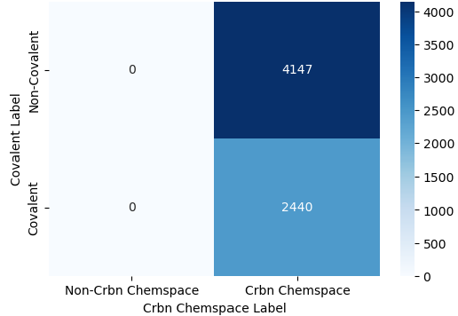
While chemical identification is frequently used in toxicology to flag hazardous substances, I applied it here to distinguish covalent CRBN candidates using Machine Learning (ML). Since I had previously annotated the common covalent warheads (examples in Figure 7), the purpose was to develop a model that captures the "chemist's intuition" — automating the recognition of these specific modalities within the CRBN-binding context.
In practical cheminformatics, success often depends on focusing on the specific chemical domain. During data preparation, I initially experimented by including covalent molecules from other Enamine libraries unrelated to CRBN (lower left, Figure 20). However, I found that this "out-of-domain" data just acted as noise - Adulterating positives for general covalency that were negative for CRBN binding confused the model, making it difficult for the machine to extract the specific structural patterns, whether through molecular fingerprints or graph-based matrices, that define the covalent CRBN chemical space. Unless you are pursuing a large-scale transfer learning approach (which would require a massive expansion of the "non-CRBN/non-covalent" negative space as shown in upper left, Figure 20), it is generally more effective to build a lean, focused model. From my personal experience working in the biotech, a model tailored specifically to the drug discovery project at hand is often more accurate and interpretable than a generalised one.
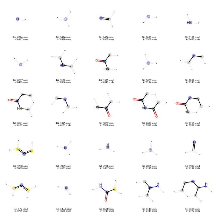
Classical Machine Learning with SVM and Tree Classifiers
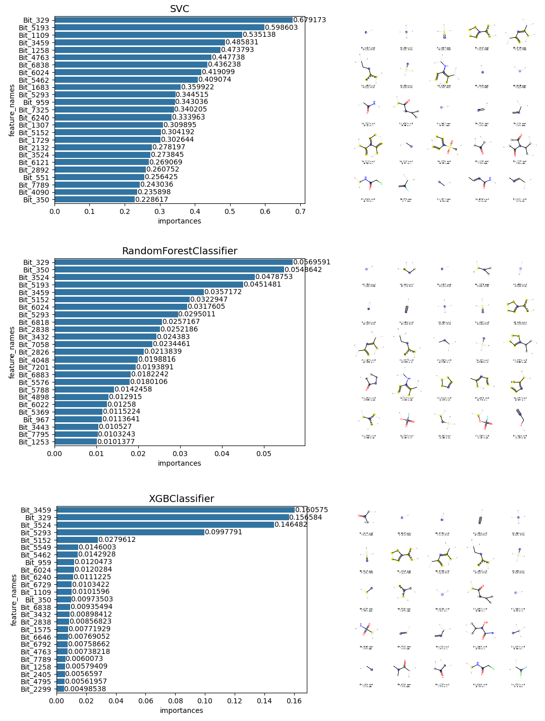
For QSAR classification tasks involving chemical spaces under 10000 compounds, classical machine learning approaches often provide superior robustness and generalisation. I initiated my study with a Support Vector Machine (SVM) utilising 8192-bit Morgan fingerprints (radius = 2, chirality ignored) based on a preliminary occupancy screening. The screening also confirmed that the majority of "on-bits" originated from the essential imide pharmacophore (Figure 21). I believe such concentration of features is not a problem for SVMs, which rather excel at defining decision boundaries in high-dimensional hyperplanes based on sparse but critical features.
To ensure generalisation as much as possible, I used a scaffold-based split, distributing unique Bemis-Murcko scaffolds into training (80%, including 20% validation) and testing (20%) sets. It attempted to prevent "data leakage" where similar analogs appear in both sets, providing a more rigorous test of the model's predictive power.
Following a hyperparameter grid search (including optimising cost, gamma, and kernel types) under 5 fold of cross-validation, the SVM model achieved near-perfect performance on the test set, with both accuracy and the Matthews Correlation Coefficient (MCC) approaching 1.0. The MCC is particularly valuable here as it provides a balanced statistical measure of precision and recall for binary classification. To validate the model's logic, I analysed the top 25 feature importances (upper, Figure 22). The results were highly interpretable: The SVM successfully prioritised bits corresponding to sulfonyl fluoride and acrylamide warheads.
I subsequently evaluated two ensemble tree-based models which often used in my work: Random Forest (RF) and eXtreme Gradient Boosting (XGBoost). After cross-validated tuning of hyperparameters such as maximum tree depth, number of estimators, and feature sub-sampling etc., both models performed exceptionally. The XGBoost model proved to be the most stable, placing significant weight on cyanamide-related bits within its decision trees (lower, Figure 22).
Nevertheless, exhaustive grid searches are computationally expensive and time-consuming. To streamline the workflow of building ML model, I implemented Bayesian optimisation using the Optuna module (Text 23) following the tip given by my Claude agent. By iterating 100 times over just a few hours, the algorithm identified an XGBoost configuration that classified the entire test set correctly.
#Tuning hyperparameters of XGBoost using Optuna based on Bayesian optimisation
import optuna

def objective(trial):
    # 1. Define the search space
    param = {
        'n_estimators': trial.suggest_int('n_estimators', 100, 1000),
        'max_depth': trial.suggest_int('max_depth', 2, 10),
        'learning_rate': trial.suggest_float('learning_rate', 0.01, 0.2, log=True),
        'subsample': trial.suggest_float('subsample', 0.5, 1.0),
        'colsample_bytree': trial.suggest_float('colsample_bytree', 0.5, 1.0),
        'gamma': trial.suggest_float('gamma', 0, 1.0),
    }
    # 2. Initialize model with suggested params
    model = XGBClassifier(**param, random_state=42, eval_metric='logloss')

    # 3. Use train data to get a score (using MCC as our metric)
    score = cross_val_score(model,
                            X_train,
                            y_train,
                            cv=5,
                            scoring='matthews_corrcoef').mean()

    return score

# 4. Create a "study" and optimize
study = optuna.create_study(direction='maximize')
study.optimize(objective, n_trials=100)
print(f"Best Params: {study.best_params}")

#Testing best XGBoost from Optuna
best_xgb_optuna = XGBClassifier(**study.best_params,
                                random_state=42,
                                eval_metric='logloss')
best_xgb_optuna.fit(X_train, y_train)
y_pred = best_xgb_optuna.predict(X_test)
acc_optuna = accuracy_score(y_test, y_pred)
mcc_optuna = matthews_corrcoef(y_test, y_pred)
print(f"Optimised XGBoost - Test MCC: {mcc_optuna:.4f} | Test ACC: {acc_optuna:.4f}")
This approach reminded me of Markov Chain Monte Carlo (MCMC) methods used for conformational searching in molecular modelling - Both aim to locate optima (or minima) within a complex landscape without requiring an exhaustive search of all possibilities. As a physical chemist doing interdisciplinary research, this highlights a core principle of data science and engineering I have learnt so far: To find a global optimum, whether in a hyperparameter distribution or a molecular energy landscape, we do not always require ab initio physics for every trial. Instead, the synergy of sufficient high-quality data, fittable empirical paradigms (such as DFT, force-field potentials, or even just robust mathematical models), and sophisticated statistical methods can navigate us toward the "ground truth" much faster. This encloses a primary goal of AI for Science: Identifying the most efficient approximation that yields a viable solution.
Classification via Graph Neural Networks (GCN, GAT, and GIN)
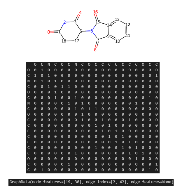
To complement the classical ML models, I also developed a deep learning pipeline using Graph Neural Networks (GNNs). Following some tutorials from DeepChem, TeachOpenCADD, and blog by Maxime Labonne, I represented each molecule in my library as a graph at the beginning. Using Thalidomide as an example (Figure 24), the chemical structure is encoded into an adjacency matrix representing bonding connectivities (edges) between atoms (nodes). With DeepChem’s featuriser, I converted these structures into three sub-matrices: node features, edge index, and edge features. For this study, the edge features were dropped because the node features implicitly capture bonding environments and they would be updated and aggregated for the awareness of edge type in most standard message-passing algorithms as far as I know. Furthermore, since we are not predicting bond-specific properties or generating alternative bonds, simplifying the graph to a node-edge-index format reduces computational redundancy without sacrificing much accuracy.
Admittedly, deep learning is often viewed as a "black box" by many computational chemists including myself who was not educated professionally with advanced mathematics. Without a formal background in linear algebra, I used the recent Christmas holiday to familiarise myself with PyTorch and modularise the following workflow based on my experience of software engineering experience as well as AI using proficiency:
1. Graph Featurisation, Collate, Scaffold-based Splitting of Training/Validation/Test Sets and Dataloader Preparation in Batch.
2. Epoch-based Training using Backpropagation with the Adam Optimiser and Binary Cross Entropy (BCE) loss for classification.
3. Regularisations including Dropout and Weight Decay to prevent overfitting on our relatively small dataset (< 10000).
4. Evaluation using MCC as the primary metric for binary classification performance.
I evaluated three distinct architectures: Graph Convolutional Network (GCN), Graph Isomorphism Network (GIN) and Graph Attention Network (GAT) (Text 25). Both GCN and GIN were inspired from TeachOpenCADD tutorial while GAT was proposed by my Gemini agent. While some architectural choices (such as layers and readout functions) might be refined further by a more experienced data scientist, I leaned on a recent industry insight from GSK: In QSAR studies, GNN architecture is often less critical than rigorous hyperparameter optimisation and feature engineering (the DOI in reference). With the deepchem graph featurised from RDKit canonical SMILES string (i.e., default tautomer but ignoring chirality), I decided to focus on tuning hyperparameters in order to maximise model performances on the classification of CRBN ligand modalities.
import torch
import torch.nn as nn
import torch.nn.functional as Fun
from torch.nn import Linear, Sequential, BatchNorm1d, ReLU
from torch_geometric.nn import GCNConv, GINConv, GATConv, global_mean_pool, global_add_pool

# Set device to GPU RTX5070 in Hao's laptop
device = torch.device("cuda" if torch.cuda.is_available() else "cpu")

# Common hyperparameters to be tuned later
HIDDEN_DIM = 32
BATCH_SIZE = 64
LEARNING_RATE = 0.001
# Some regularisation parameters to prevent overfitting issue given limited crbn data < 10000
DROPOUT_P = 0.5
WEIGHT_DECAY = 1e-4
EPOCHS = 100
EARLY_STOP_PATIENCE = 5
# Initial random seed which will be varied 2 more times (21, 0) for robustness testing
RANDOM_SEED = 42

# Define GNN architectures: GCN, GIN, and GAT
class GCN(torch.nn.Module):
    def __init__(self, in_features, dim_h):
        super().__init__()
        # GCNConv layers for graph convolutional operations
        self.conv1 = GCNConv(in_features, dim_h)
        self.conv2 = GCNConv(dim_h, dim_h)
        self.conv3 = GCNConv(dim_h, dim_h)
        self.lin = torch.nn.Linear(dim_h, 1)
    def forward(self, graphs_in):
        # Normalize input to a list of graph objects
        graphs_list = list(graphs_in)
        x_list = []
        edge_list = []
        batch = []
        node_offset = 0
        # Build concatenated Tensors (x, edge_index, batch vector)
        for i, g in enumerate(graphs_list):
            # Convert node features and edge index to 2 tensors and move them to device (GPU/CUDA)
            nf = torch.tensor(g.node_features, dtype=torch.float32).to(device)
            ei = torch.tensor(g.edge_index, dtype=torch.long).to(device)
            # Shift edge indices by the current node offset
            edge_list.append(ei + node_offset)
            x_list.append(nf)
            # Create batch vector for this graph (all nodes get the same graph index)
            n_nodes = nf.shape[0]
            batch.append(torch.full((n_nodes,), i, dtype=torch.long, device=device))
            node_offset += n_nodes
        # Concatenate all features, edges, and batch vectors
        x = torch.cat(x_list, dim=0)
        e = torch.cat(edge_list, dim=1)
        batch = torch.cat(batch, dim=0)
        # GCN layers with ReLU activations
        x = self.conv1(x, e)
        x = x.relu()
        x = self.conv2(x, e)
        x = x.relu()
        x = self.conv3(x, e)
        # Global Pooling with mean aggregation for GCN graph-level prediction
        x = global_mean_pool(x, batch)
        # Readout layer
        x = Fun.dropout(x, p=DROPOUT_P, training=self.training)
        x = self.lin(x) # Output logits (unscaled)
        return x.squeeze(-1) # Squeeze to shape [batch_size]

class GIN(torch.nn.Module):
    def __init__(self, in_features, dim_h):
        super(GIN, self).__init__()
        # Add BatchNorm for GIN stability
        self.conv1 = GINConv(
            Sequential(Linear(in_features, dim_h), BatchNorm1d(dim_h), ReLU(),
                      Linear(dim_h, dim_h), BatchNorm1d(dim_h), ReLU())
        )
        self.conv2 = GINConv(
            Sequential(Linear(dim_h, dim_h), BatchNorm1d(dim_h), ReLU(),
                      Linear(dim_h, dim_h), BatchNorm1d(dim_h), ReLU())
        )
        self.conv3 = GINConv(
            Sequential(Linear(dim_h, dim_h), BatchNorm1d(dim_h), ReLU(),
                      Linear(dim_h, dim_h), BatchNorm1d(dim_h), ReLU())
        )
        self.lin = Linear(dim_h, 1)
    def forward(self, graphs_in):
        graphs_list = list(graphs_in)
        x_list = []
        edge_list = []
        batch = []
        node_offset = 0
        for i, g in enumerate(graphs_list):
            nf = torch.tensor(g.node_features, dtype=torch.float32).to(device)
            ei = torch.tensor(g.edge_index, dtype=torch.long).to(device)
            edge_list.append(ei + node_offset)
            x_list.append(nf)
            n_nodes = nf.shape[0]
            batch.append(torch.full((n_nodes,), i, dtype=torch.long, device=device))
            node_offset += n_nodes
        x = torch.cat(x_list, dim=0)
        e = torch.cat(edge_list, dim=1)
        batch = torch.cat(batch, dim=0)
        # GIN layers with MLPs and BatchNorm
        x = self.conv1(x, e)
        x = self.conv2(x, e)
        x = self.conv3(x, e)
        # Global Pooling with sum aggregation for GIN graph-level prediction
        x = global_add_pool(x, batch)
        x = Fun.dropout(x, p=DROPOUT_P, training=self.training)
        x = self.lin(x)
        return x.squeeze(-1)

class GAT(torch.nn.Module):
    def __init__(self, in_features, dim_h, heads=3):
        super(GAT, self).__init__()
        # GATConv layers for graph attention operations
        self.conv1 = GATConv(in_features, dim_h, heads=heads, concat=True)
        self.conv2 = GATConv(dim_h * heads, dim_h, heads=heads, concat=True)
        self.conv3 = GATConv(dim_h * heads, dim_h, heads=1, concat=False)
        self.lin = Linear(dim_h, 1)
    def forward(self, graphs_in):
        graphs_list = list(graphs_in)
        x_list = []
        edge_list = []
        batch = []
        node_offset = 0
        for i, g in enumerate(graphs_list):
            nf = torch.tensor(g.node_features, dtype=torch.float32).to(device)
            ei = torch.tensor(g.edge_index, dtype=torch.long).to(device)
            edge_list.append(ei + node_offset)
            x_list.append(nf)
            n_nodes = nf.shape[0]
            batch.append(torch.full((n_nodes,), i, dtype=torch.long, device=device))
            node_offset += n_nodes
        x = torch.cat(x_list, dim=0)
        e = torch.cat(edge_list, dim=1)
        batch = torch.cat(batch, dim=0)
        # GAT layers with attention mechanism
        x = self.conv1(x, e)
        x = x.relu()
        x = self.conv2(x, e)
        x = x.relu()
        x = self.conv3(x, e)
        # Global Pooling with mean aggregation for GAT graph-level prediction
        x = global_mean_pool(x, batch)
        x = Fun.dropout(x, p=DROPOUT_P, training=self.training)
        x = self.lin(x)
        return x.squeeze(-1)
As shown in the grid search results (Figure 26), all three GNN models could identify covalent CRBN modulators with exceptional precision and recall (MCC > 0.95). Nevertheless, the GIN model demonstrated the most robust MCC stability across varying hyperparameters. By utilising Bayesian optimisation alternatively, an optimal GIN configuration was more quickly found (Hidden Dim: 16, Batch Size: 16, Learning Rate: 0.001) that achieved an MCC up to 0.98. It is obvious that both classical ML and GNN approaches proved highly capable of handling this classification task to identify those covalent modalities in the CRBN chemical space. Then how about regression modeling?

Regression Task on Electrophilicity
In covalent drug discovery, quantifying reactivity is a primary challenge for medicinal chemists. While biophysical assays can measure kinetic parameters such as k_inact/K_I for detailed mechanistic study in the protein environment, high-throughput alternatives like the Glutathione (GSH) reactivity assay provide a shortcut to evaluate a molecule's propensity for the cysteine engagement. Computationally, this reactivity can be even roughly estimated through the lens of frontier molecular orbital (FMO) theory — specifically by calculating HOMO (Highest Occupied Molecular Orbital) and LUMO (Lowest Unoccupied Molecular Orbital) energies. Having previously annotated our CRBN chemical space into covalent and non-covalent classes, I set out to determine if these empirical labels could be characterised and quantified through rigorous electronic descriptors.
Quantum Chemical Calculations
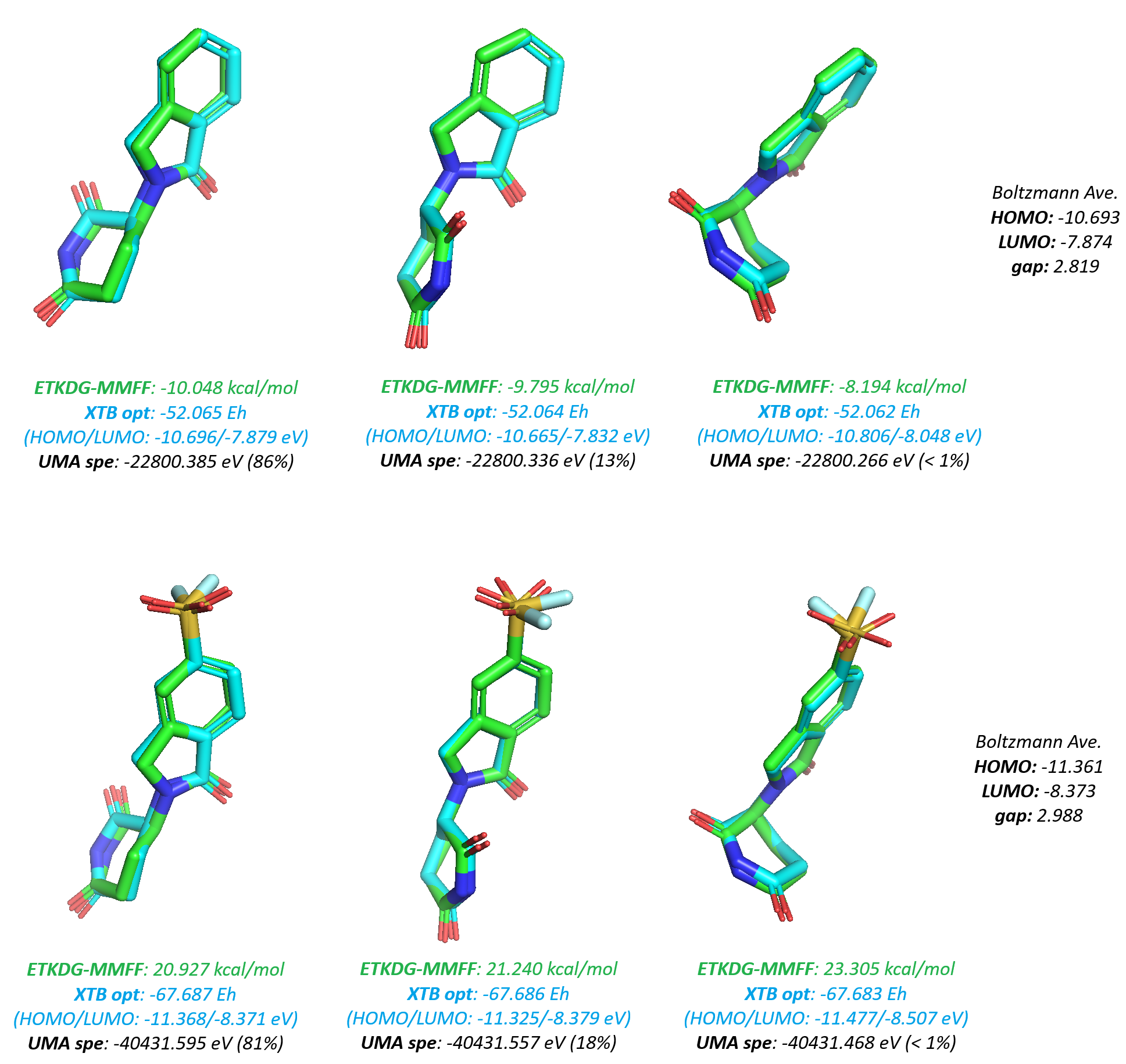
To calculate molecular electronic properties at scale, I instructed my AI agent to develop a workflow using a "conformationally dependent" statistical QM approach. The pipeline begins with stereo-isomers enumeration, ETKDG (MMFF) conformational sampling, followed by xTB geometry optimisation, and culminates in single-point energy calculations using the UMA (Universal Machine Learning Approximation) model. Final properties were derived through Boltzmann averaging over the resulting low-energy ensembles in vacuum (Figure 27). This semi-empirical approach serves as a pragmatic compromise for screening over 10000 hit candidates: It avoids the extreme computational cost of full DFT or MD simulations while maintaining a level of accuracy superior to classic density functionals or force fields, thanks to the integration of atomic neural network potentials (NNP) - as supported by the study in my previous blog.
Following the computational screening, a comparison of the electronic profiles between the covalent and non-covalent classes revealed statistically significant differences (p < 0.05 via both Mann-Whitney U and t-tests). Those covalent species generally exhibited lower LUMO energies, higher HOMO energies, and smaller HOMO-LUMO gaps (Figure 28). Furthermore, the distribution of the electrophilicity index (ω), calculated using the following relationship, was markedly higher for the covalent class:
\[\omega = \frac{(E_{H} + E_{L})^2}{4(E_{L} - E_{H})}\]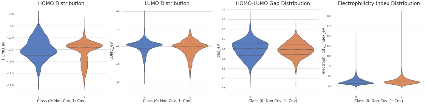
Despite these trends, molecular-level QM features alone are often insufficient for high-confidence classification of covalency - A finding consistent with research from Bayer (the DOI in reference). True predictive power likely requires fragment-specific descriptors, such as Fukui indices on the warhead atoms and further calculated transition-state activation energies for the nucleophilic addition. However, because the LUMO energy is the primary orbital for accepting nucleophilic electrons and its distribution in our dataset closely follows a Gaussian-like profile (second plot, Figure 28), I selected it as the target variable for our regression modelling next.
Benchmarking ML Models for LUMO Prediction
The regression modelling workflow followed a similar logic to the previous classification task, with a critical difference in the loss function: Mean Squared Error (MSE) was implemented to fit and predict continuous energy values. Another significant adjustment was made regarding molecular featurisation. Since our target, QM-calculated LUMO energies, is derived from conformational analysis of specific stereoisomers, this time I incorporated stereochemical features into both the 1D Morgan fingerprints and the 2D graph matrices. By including chirality, I aimed to reduce "structural noise" and increase physical relevance, allowing the models to better recognise the subtle patterns that govern 3D-dependent quantum chemical properties.
Using the same scaffold-based training/test split and a combination of validated grid search and Bayesian optimisation, I benchmarked the regression performance across 6 pre-trained and tuned architectures again: SVM, RandomForest, XGBoost, GCN, GAT and GIN (Table 29).
| Regression Models | Molecular Features | Test MSE | Test MAE | Test R2 | Running Time | Model Size |
|---|---|---|---|---|---|---|
| SVM | Morgan - 8192 bits, 2 radius & include chirality | 0.0408 | 0.1409 | 0.7269 | Slow | .pkl file ~ 600MB |
| RandomForest | Morgan - 8192 bits, 2 radius & include chirality | 0.0530 | 0.1613 | 0.6454 | Medium | .pkl file ~ 100MB |
| XGBoost | Morgan - 8192 bits, 2 radius & include chirality | 0.0414 | 0.1452 | 0.7232 | Fast | .pkl file ~ 500KB |
| GCN | Graph (node features + edge index) | 0.0497 | 0.1716 | 0.6677 | Fast (GPU) | .pth file < 10KB |
| GAT | Graph (node features + edge index) | 0.0476 | 0.1656 | 0.6818 | Fast (GPU) | .pth file ~ 12KB |
| GIN | Graph (node features + edge index) | 0.0409 | 0.1447 | 0.7266 | Fast (GPU) | .pth file ~ 12KB |
The results highlight an interesting trend: For our focused CRBN dataset, the graph models showed no significant improvement over classical ML models in terms of R2 score (coefficient of determination). Both SVM and GIN regressions were optimised to produce a strong fit (Test R2 up to 0.725) on the QM-calculated LUMO values. However, The GIN architecture offered a distinct engineering advantage: The training was significantly faster due to GPU acceleration (also save RAM compared to classical models using CPU), and the final model deployment is more efficient, requiring only the saved parameter dictionary (remember that SVM utilise RBF kernel). Meanwhile, XGBoost also proved to be a standout performer - high stability, minimal overfitting, lightweight storage as well as interpretable reasoning - making it an excellent alternative for rapid re-usage in production pipelines.
Testing Generative AI
With a robust foundation of public data, virtual screening hits, and validated QSAR models as discussed above, I transitioned to the final phase: De Novo Molecular Generation. From the perspective of computational medicinal chemistry, I would seek the answer for two objectives: Could these models further diversify our CRBN chemical space? Are they able to reliably "invent" novel, drug-like covalent candidates?
I first evaluated smilesRNN, a recurrent neural network (RNN)-based generative workflow developed by the MorganCThomas/Nxera team. By processing SMILES strings as sequences of tokens, the model learns the underlying grammar of chemical structures and performs targeted generation. After some reading (the DOI in reference) and trials with command line wrapper, I explored two primary strategies:
Direct Prior Training: Training a “Prior” model exclusively on our curated CRBN chemical space, then sampling from this learned distribution to generate closely related analogs.
Available Prior Fine-Tuning: Taking a large, pre-trained prior (e.g., latest reinvent model based on the entire ChEMBL database) and fine-tuning it on our focused CRBN dataset to bias the output toward the desired scaffold diversity.
I also implemented the latest REINVENT4 platform from AstraZeneca. Similar to the prior fine-tuning approach of smilesRNN, it offers more sophisticated transfer learning (TL) and reinforcement learning (RL) frameworks. By configuring .toml file in each step, multi-objective scoring functions could be integrated — including SMARTS filters for medicinal chemistry alerts (e.g., PAINS), QED for drug-likeness, and even external QSAR models etc.
- TL & RL with Scoring: Through transferring knowledge from a large prior to the CRBN-specific space, an appropriate agent was chosen to sample a “neighbouring” chemical space under reasonable constraints.
A key technical challenge identified by my Gemini agent was that the publicly available reinvent prior model recognises only 59 tokens from SMILES string. This vocabulary excludes stereochemical labels like '@' or explicit hydrogens such as '[H]' - This means our current CRBN dataset must be pre-processed to ensure token compatibility before the generative RL.
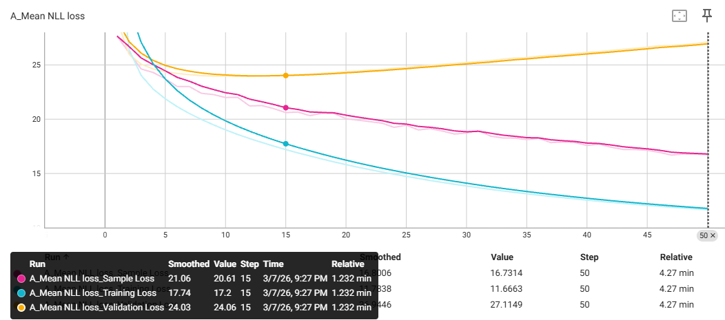
Meanwhile, in the TL stage for building agents, I employed a training/validation split and monitored the Negative Log-Likelihood (NLL) as the loss function. The metric of NLL was announced to evaluate how well the agent model is learning to mimic the specific grammar of our CRBN chemical space (Figure 30). Without any experience on how it would affect the subsequent RL phase, I decided to test two specific agents trained from REINVENT4:
a. The final agent where all sample loss is optimised to a minimum (step 50)
b. The checkpoint agent when the validation loss reached to a stable plateau (step 15) - persumably offering better structural diversity before over-fitting to the training set?
Comparative Performance and Scaffold Diversity
The Table 31 summarises the generative capacity of each approach, constrained by my tailored hierarchical post-processing pipeline for enumerating CRBN chemical space effectively. To ensure a high confidence in the identification of covalency, I employed a dual-classifier consensus: Only molecules flagged as positives/negatives by both of my XGBoost and GIN models were prioritised - This multi-model validation was found to significantly reduces artifacts in determining two modalities.
| Approach | Targeted ‘Mols’ | Valid Smiles | Novel Mols | Mols with Imide Substructure | Mols without ‘PAINS’ | Mols QED > 0.5 | Non/Covalent Candidates Passing both XGBoost & GIN Classifiers together |
|---|---|---|---|---|---|---|---|
| smilesrnn approach 1 | 10000 | 7142 | 6140 | 5899 | 5490 | 5181 | 3910/1171 |
| smilesrnn approach 2 | 10000 | 9917 | 5050 | 4627 | 4413 | 4090 | 3048/1006 |
| reinvent4 approach 3a | 30000 | 23089 | 22276 | 3188 | 3007 | 2861 | 2489/343 |
| reinvent4 approach 3b | 30000 | 26028 | 25738 | 3373 | 3121 | 2951 | 2582/329 |
Here are my observations and assumptions from the test above:
Distribution Fidelity: Both smilesRNN approaches (Direct Prior and Fine-Tuning) showed high fidelity to the training set. For example, the ratio of generated non-covalent to covalent candidates (3~4:1) closely mirrors the original distribution, suggesting these models might be suitable for SAR exploitation tasks (such as hit expansion or lead optimisation).
Scaffold Innovation: The REINVENT4 demonstrated a significant ‘drop-off’ during my check with imide pharmacophore. While this results in lower efficiency to generate ‘secure’ hits, it indicates a higher tendency for de novo innovation. More bioisosteres or alternative cores could be explored for new ideas beyond the imide-heavy bias based on training set.
Access to Drug-likeness: All protocols are able to produce some high-quality candidates (QED > 0.5 and no undesired alert) for potential drug development in spite of ignored stereochemistry. I think smilesRNN is more user friendly without the need to supply explicit reward functions as configured in .toml file for RL stage of REINVENT4 (Note: I have not tried any extra function such as MolScore or PromptSMILES that recently added on the base of smilesRNN).
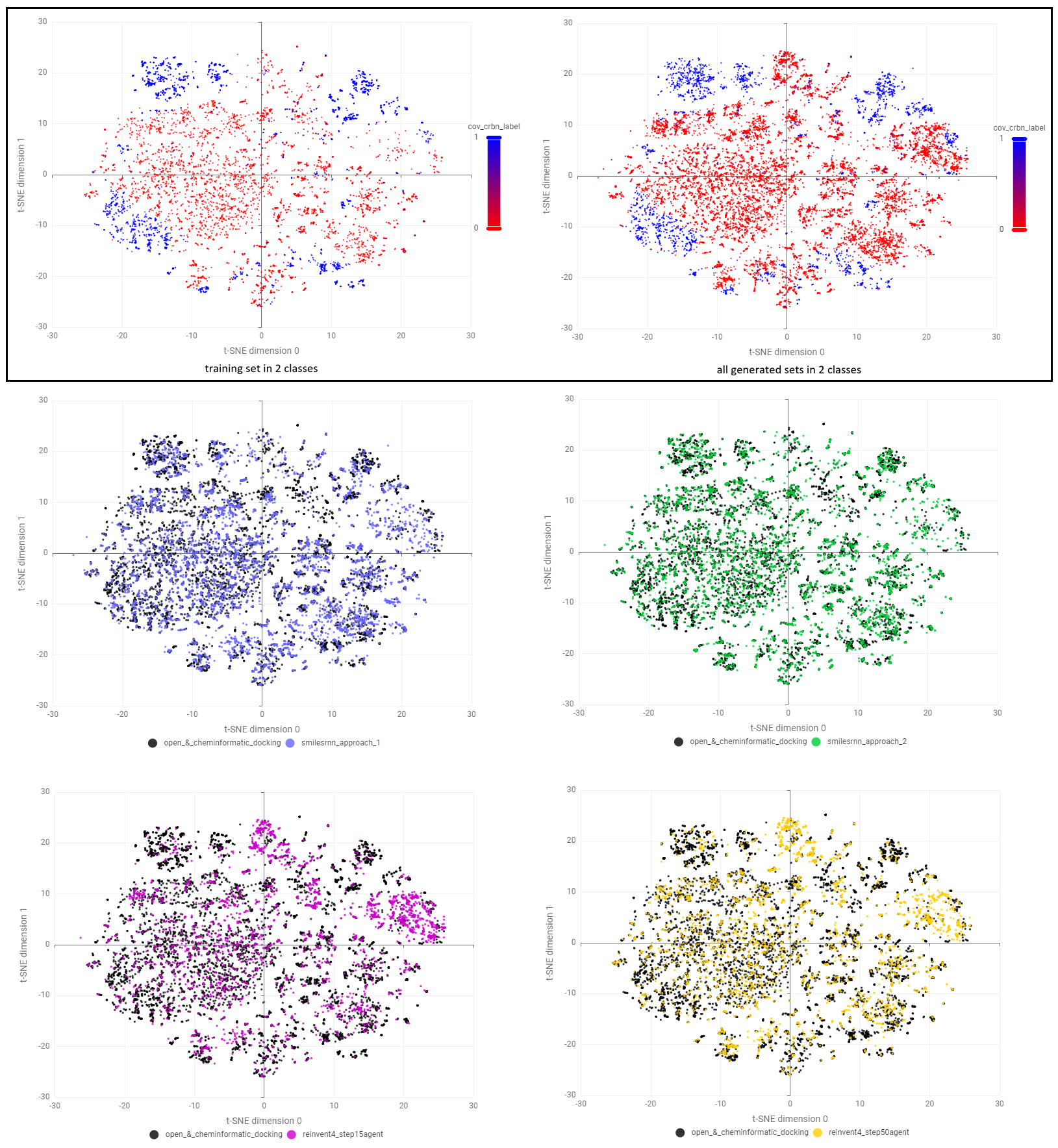
To check the final selected space in detail, some t-SNE plots were projected from two perspectives - class of covalency and source of datasets (Figure 32). According to the upper row, our CRBN chemical space was enriched generally with all generative models following the filtration. Different from smilesRNN where analogs were mainly filled around existing clusters, REINVENT4 created a plenty of candidates in sparse regions (top and right corners of t-SNE plot) especially for noncovalent class. Interactive investigation of structures in KNIME revealed that REINVENT4 preferentially explore the space of 'suspicious molecular glues' with Phenyl Dihydrouracil (PD) and Phenyl 3-substituted-Glutarimide (P3G) which are rare in our training set. I assume this is due to the addition of penalty weight on stereo-centres in reward functions that reduce the generation of chiral cores such as Phenyl 2-substituted-Glutarimide (P2G) in RL process.
Prioritising AI-generated CRBN Covalent Candidates via Property-based Optimisation
With a large pool of AI-generated structures even after post-processing, the next challenge is prioritisation. While physics-based structural modelling (including docking, MD and even FEP workflows) is a standard procedure as I demonstrated earlier and in previous blog, it becomes a bottleneck when dealing with many novel scaffolds generated by AI - There is a plenty of structures (e.g., warhead tautomers) that are hard to be prepared with a set of sidechain transformations before the covalent docking. Even with some positively docked structures, further MD simulation of covalent modalities also require complex force-field parameterisation which are time-consuming against the essence of screening.
Based on my industrial CADD experience, when SBDD is impracticable, the property-based optimisation strategy become an alternative choice in LBDD. For this case of discovering covalent CRBN modulators, I believe binding affinity, reactive kinetics, potency and efficacy are only half the battle; Physicochemical, ADME, and DPMK properties are equally critical for ensuring that a molecule can reach its target in vivo.
For the large-scale virtual screening, I think three molecular descriptors are highly indicative to guide above performances at late stage:
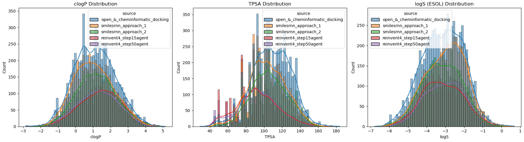
logP (Logarithm of the Partition coefficient) - Its ideal range is likely between 1.0 and 3.5 for the desired lipophilicity (logD if pH considered). Using RDKit’s fragment-based calculation is a robust baseline for this domain.
TPSA (Topological Polar Surface Area) - As a proxy for permeability and oral bioavailability, I monitored TPSA with an upper threshold of 130 Ų. While such 2D-based value is a “quick and dirty” metric, it remains a gold standard for initial prioritisation in MG and PROTAC design.
logS (Logarithm of Water Solubility) - Such value above -4.0 could indicate sufficient distribution in aqueous environment. For corresponding calculation, I prefer to use ESOL approach (Estimated SOLubility) - A reliable linear regression model based on clogP, MW, nRotB and Aromatic proportion features, as established by Delaney and refined by Pat Walters.
As shown in the distribution analysis (Figure 33), the majority of our generated candidates after post-processing fall within these desired physicochemical regions. Interestingly, smilesRNN (especially without a global prior) tended to generate more polar, hydrophilic molecules that closely matched the training set's local distribution. In contrast, REINVENT4 explored a more narrow range of lipophilic "sweet spot".
To visualise some of novel covalent products meeting all three criteria, I used mols2grid module to list AI-generated candidates that passed the dual-classifier check (XGBoost+GIN) and maintained high drug-likeness (QED > 0.67). As shown in Video 34, the resulting 82 final structures represent a highly diverse chemical space including:
Novel PD-based CRBN molecular glues
Imide in 7-membered rings (albeit with one exception of open imide at the first)
All sets of reactive warhead as expected
I believe this AI-enhanced chemical space derived from open and cheminformatic docking dataset, combined with my rational supervision through property-based optimisation strategy, has yielded a rich pipeline of covalent CRBN-binding candidates ready for synthetic, structual and biological validations if any reader would like to explore...
Video 34. The monitored generative AI product of some drug-like candidates in covalent CRBN chemical space, as shown by mols2grid module with RDKit-calculated properties.Summary and Outlook
In this blog, I explored the CRBN chemical space with a focus on sparse covalent modalities. It highlights the powerful synergy between classical computational chemistry, data-driven cheminformatics and modern AI workflows. By moving from comprehensive data curation and into the physics/ML-integrated drug design, we have transformed raw, imbalanced, unlabelled public datasets to productive libraries refined for drug discovery and development practically. I think there are some key takeaways from this blog:
We must addrees the bias when deal with any dataset in the public. It would be benefitial to enrich the chemical space with specialised libraries and patent mining correspondingly. With human-level cheminformatic skills, this enabled me to design and develop potential candidate pool targeting covalent residues in the space of CRBN modulators.
Virtual screening is more than simply doing the docking. By implementing pharmacophore shape constraints and Shortest Bonding Pathlength (SBP) filters, I ensured that our covalent “inventions” were target-focused and structurally plausible within CRBN and interfaces for IKZF2 and WIZ.
For structural identification and regressive analysis, satisfactory approximation, generalisation and automation could be achieved by most fine-tuned ML models based on well-distributed data. The QSAR modelling in my study domain is not very sensitive to feature type or architecture choice, no matter it is classical fingerprint tree or popular graph neural network… I believe both data quality through annotation or QM and model deployability in engineering are overlooked factors to consider for drug discovery industry.
From my perspective as application scientist, AI molecular generation with RL represents a promising future direction that now established on appropriate data/prior of available chemical space together with the generative agent rewarded by desired metrics. For computational drug designer at the moment, it is still necessary to keep monitoring these generative progress with a human mindset of biological targets in SBDD physics as well as molecular properties for ADME and DPMK.
Data, Code and Model Availability
Reference and Acknowledgement
This personal blog post was made possible with excellent open-source software, database, models, toolkits, platforms and publications below under corresponding licenses:
RDKit: The fundamental cheminformatic tookits used for chemical data processing, Murcko scaffold-based splitting, Morgan fingerprints generation, ETKDG conformer search, descriptor calculations etc. in this blog.
KNIME: The pipeline platform used here for tabular cheminformatic database curation, analysis and visualisation.
Enamine: The link for latest molecular glues library in their commercial store.
DOI: The research of covalent Cereblon modulators published by Lyn Jones group in Dana-Farber.
DOI: The QSAR modelling study with GNN architectures published from GSK.
TechOpenCADD: The series of deep learning tutorials that inspired GNN works for QSAR study here.
DeepChem: The deep learning module used to prepare and featurise chemical graph data in QSAR.
Pytorch: The foundation open-source deep learning framework used in GNN modelling.
Scikit-learn: The platform for classical ML models in QSAR study.
Optuna: The framework for hyperparameter optimisation and model tuning specifically with Bayesian algorithm.
DOI: The paper of QM computation for estimating electrophilicty with applications to covalent inhibitors published from Bayer
XTB: The semi-empirical quantum mechanics program used here for conformational geometry optimisations and electronic property calculations.
FAIRCHEM: The Meta’s UMA model as SOTA machine-learning force field used here for single-point energy calculation and Boltzmann averaging of conformation-dependent electronic properties.
AutoDock-GPU: The GPU version of AutoDock 4 used here for covalent docking with flexible sidechain mode.
smilesRNN: The generative scripts released by MorganCThomas/Nxera team with their publication DOI.
REINVENT4: The latest generative platform developed from AstraZeneca with their publication DOI.
Gemini & Claude Two latest AI agents integrated in my VSCode/GitHub Copilot Pro account for coding workflow assistance and blog writing refinement.
Disclaimer
The entirety of the content, methodologies, analyses, and conclusions presented in this personal blog post are solely the contribution of myself as the author, and are based exclusively on open-source, non-commercial-use software and publicly available data. This work is intended purely for academic and educational use and is not related to, reflective of, or affiliated with the work, practices, or proprietary information of any of my current or previous employers.
Additional Note
Due to few unforeseen events in my career and family, I would pause the update for this series of technical blog for a period of time. Meanwhile, there are some emerging matters I need to prioritise sooner rather than later - gain professional knowledge in ADME/DMPK, practice communication for CADD technical leadership and software product management in industry, stick at body maintenance for personal health and take care on the next generation etc... all of which are becoming even more important nowadays in a world with AGI.